Friday, April 4

Censoring Specification

Without much loss of generality we will limit the discussion here to right-censoring. We define an indicator variable $D_i$ such that $$D_i = \begin{cases} 1, & \text{if the $i$-th observation is not censored}, \\ 0, & \text{if the $i$-th observation is censored}. \end{cases}$$ The variable $D_i$ can be viewed as another response variable which depends on the actual time to event, $T_i$, as well as whatever is responsible for the censoring. In what follows we will let $t_i$ and $d_i$ denote observed values of $T_i$ and $D_i$ respectively.

Let $t_i$ be the actual time-till-event if $d_i = 1$, and the lower-bound on the time-till-event if $d_i = 0$ so that the actual time-till-event is greater than or equal to $t_i$. Under certain assumptions about how censoring occurs, the likelihood function is $$L = \prod_{i=1}^n f(t_i)^{d_i}P(T_i \ge t_i)^{1-d_i}.$$ where $f(t_i)$ is the probability density function of $T_i$, and $P(T_i \ge t_i)$ is the probability that $T_i$ is at least $t_i$ (this is also called the survival function). Note that $$f(t_i)^{d_i}P(T_i \ge t_i)^{1-d_i} = \begin{cases} f(t_i), & \text{if $d_i = 1$ (i.e., not censored)}, \\ P(T_i \ge t_i), & \text{if $d_i = 0$ (i.e., censored)}, \end{cases}$$ so the indicator variable $d_i$ simply selects the appropriate term for computing the likelihood of an observation depending on whether or not it was censored.

library(survival) # for leukemia and survreg
head(leukemia) # status=1 if remission ended at that time, status=0 if right-censored

  time status          x
1    9      1 Maintained
2   13      1 Maintained
3   13      0 Maintained
4   18      1 Maintained
5   23      1 Maintained
6   28      0 Maintained

m <- survreg(Surv(time, status) ~ x, dist = "lognormal", data = leukemia)
summary(m)$table

                Value Std. Error      z        p
(Intercept)     3.579      0.285 12.571 3.04e-36
xNonmaintained -0.724      0.380 -1.905 5.68e-02
Log(scale)     -0.145      0.170 -0.858 3.91e-01

leukemia$censored <- factor(leukemia$status, labels = c("yes","no"))
head(leukemia)

  time status          x censored
1    9      1 Maintained       no
2   13      1 Maintained       no
3   13      0 Maintained      yes
4   18      1 Maintained       no
5   23      1 Maintained       no
6   28      0 Maintained      yes

m <- survreg(Surv(time, censored == "no") ~ x, dist = "lognormal", data = leukemia)
summary(m)$table

                Value Std. Error      z        p
(Intercept)     3.579      0.285 12.571 3.04e-36
xNonmaintained -0.724      0.380 -1.905 5.68e-02
Log(scale)     -0.145      0.170 -0.858 3.91e-01

leukemia$ysurv <- Surv(leukemia$time, leukemia$censored == "no")
head(leukemia)

  time status          x censored ysurv
1    9      1 Maintained       no     9
2   13      1 Maintained       no    13
3   13      0 Maintained      yes   13+
4   18      1 Maintained       no    18
5   23      1 Maintained       no    23
6   28      0 Maintained      yes   28+

exp(cbind(coef(m),confint(m)))

                      2.5 % 97.5 %
(Intercept)    35.833 20.51  62.60
xNonmaintained  0.485  0.23   1.02

leukemia$x <- relevel(leukemia$x, ref = "Nonmaintained")
m <- survreg(Surv(time, status) ~ x, dist = "lognormal", data = leukemia)
summary(m)$table

             Value Std. Error      z        p
(Intercept)  2.854      0.254 11.242 2.55e-29
xMaintained  0.724      0.380  1.905 5.68e-02
Log(scale)  -0.145      0.170 -0.858 3.91e-01

exp(cbind(coef(m),confint(m)))

                   2.5 % 97.5 %
(Intercept) 17.36 10.556  28.56
xMaintained  2.06  0.979   4.35

Interval-Censoring

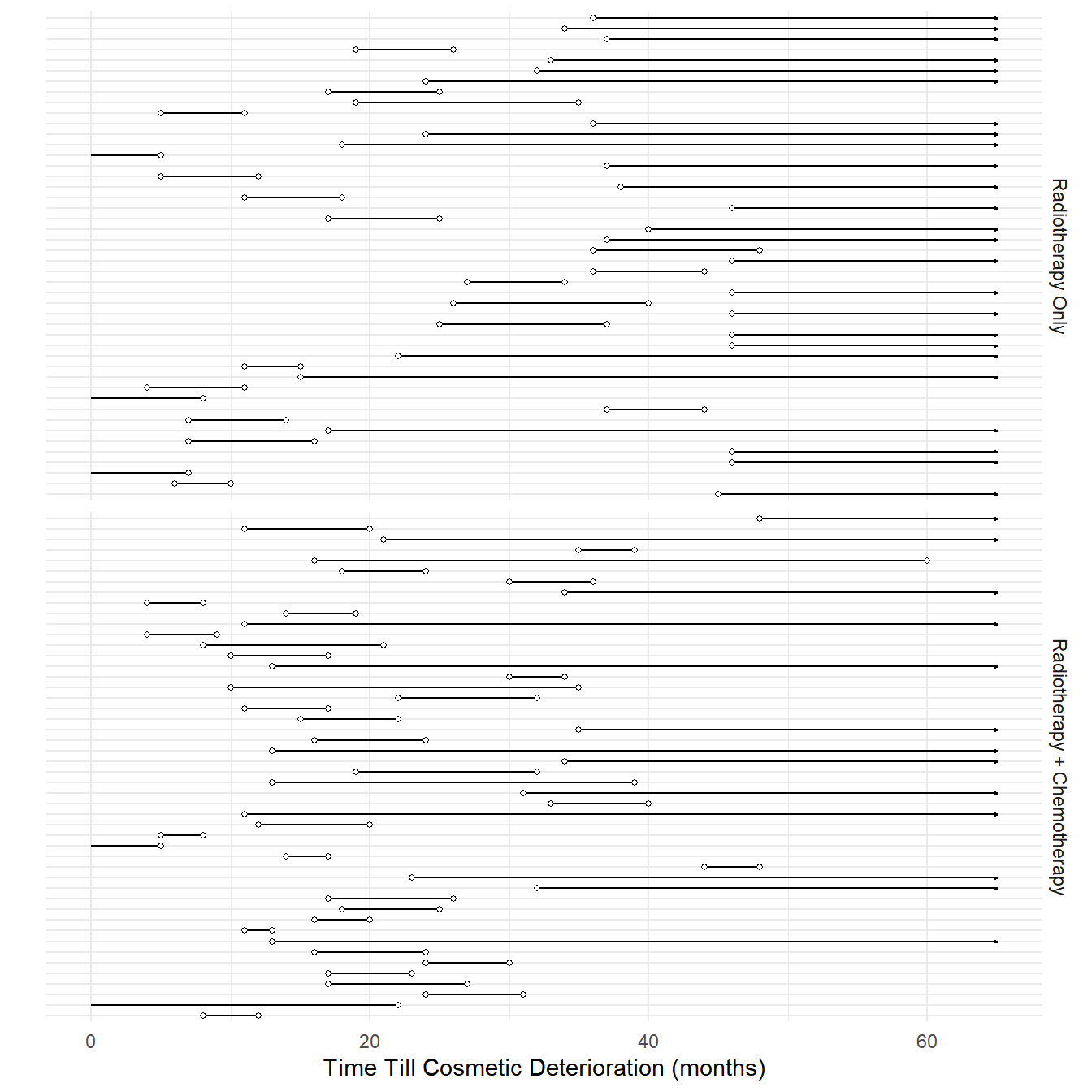
Interval censoring occurs when $T_i$ is only known to be between two numbers such that $a < T_i < b$ where $0 \le a < b \le \infty$. Note that right-censoring is a special case where $b = \infty$, and left-censoring is a special case where $a = 0$.

Example: Consider the following data from a study of the time till cosmetic deterioration for breast cancer patients undergoing radiotherapy alone versus radiotherapy and chemotherapy.

library(mable) 
head(cosmesis, 10)

   left right treat
1    45    NA    RT
2     6    10    RT
3     0     7    RT
4    46    NA    RT
5    46    NA    RT
6     7    16    RT
7    17    NA    RT
8     7    14    RT
9    37    44    RT
10    0     8    RT

Note that these data include left-censoring, interval-censoring, and right-censoring). Using the Surv function to specify censoring requires that lower bounds of 0 and upper bounds of $\infty$ be replaced with NA.

cosmesis$left <- ifelse(cosmesis$left == 0, NA, cosmesis$left)
head(cosmesis, 10)

   left right treat
1    45    NA    RT
2     6    10    RT
3    NA     7    RT
4    46    NA    RT
5    46    NA    RT
6     7    16    RT
7    17    NA    RT
8     7    14    RT
9    37    44    RT
10   NA     8    RT

tail(cosmesis, 10)

   left right treat
85   14    19   RCT
86    4     8   RCT
87   34    NA   RCT
88   30    36   RCT
89   18    24   RCT
90   16    60   RCT
91   35    39   RCT
92   21    NA   RCT
93   11    20   RCT
94   48    NA   RCT

It is also useful to note that you can accommodate an observation that is not censored by specifying equal left and right interval endpoints.

We can verify the censoring specification by looking at what Surv produces.

cosmesis$y <- with(cosmesis, Surv(left, right, type = "interval2"))
head(cosmesis, 10)

   left right treat        y
1    45    NA    RT      45+
2     6    10    RT [ 6, 10]
3    NA     7    RT       7-
4    46    NA    RT      46+
5    46    NA    RT      46+
6     7    16    RT [ 7, 16]
7    17    NA    RT      17+
8     7    14    RT [ 7, 14]
9    37    44    RT [37, 44]
10   NA     8    RT       8-

Now we can estimate an AFT model.

m <- survreg(Surv(left, right, type = "interval2") ~ treat,
  dist = "lognormal", data = cosmesis)
summary(m)$table

             Value Std. Error     z         p
(Intercept)  3.548      0.154 23.01 3.45e-117
treatRCT    -0.421      0.203 -2.07  3.83e-02
Log(scale)  -0.125      0.109 -1.15  2.52e-01

Applying the exponential function helps interpret the effect of the treatment.

exp(cbind(coef(m), confint(m)))

                    2.5 % 97.5 %
(Intercept) 34.739 25.680 46.995
treatRCT     0.656  0.441  0.978

Using flexsurvreg produces the same information but in one output.

library(flexsurv)

Warning: package 'flexsurv' was built under R version 4.4.3

m <- flexsurvreg(Surv(left, right, type = "interval2") ~ treat, 
  dist = "lognormal", data = cosmesis)
print(m)

Call:
flexsurvreg(formula = Surv(left, right, type = "interval2") ~ 
    treat, data = cosmesis, dist = "lognormal")

Estimates: 
          data mean  est      L95%     U95%     se       exp(est)  L95%     U95%   
meanlog        NA     3.5479   3.2457   3.8500   0.1542       NA        NA       NA
sdlog          NA     0.8821   0.7118   1.0933   0.0966       NA        NA       NA
treatRCT   0.5106    -0.4210  -0.8192  -0.0228   0.2032   0.6564    0.4408   0.9775

N = 94,  Events: 0,  Censored: 94
Total time at risk: 2089
Log-likelihood = -147, df = 3
AIC = 299

Again, it is sometimes helpful for interpretation to change the reference level when dealing with categorical explanatory varaibles.

cosmesis$treat <- relevel(cosmesis$treat, ref = "RCT")
m <- flexsurvreg(Surv(left, right, type = "interval2") ~ treat, 
  dist = "lognormal", data = cosmesis)
print(m)

Call:
flexsurvreg(formula = Surv(left, right, type = "interval2") ~ 
    treat, data = cosmesis, dist = "lognormal")

Estimates: 
         data mean  est     L95%    U95%    se      exp(est)  L95%    U95%  
meanlog      NA     3.1269  2.8558  3.3980  0.1383      NA        NA      NA
sdlog        NA     0.8821  0.7118  1.0933  0.0966      NA        NA      NA
treatRT  0.4894     0.4210  0.0228  0.8192  0.2032  1.5235    1.0230  2.2688

N = 94,  Events: 0,  Censored: 94
Total time at risk: 2089
Log-likelihood = -147, df = 3
AIC = 299

Survival Functions

The survival function is $$S(t) = P(T \ge t),$$ i.e., the probability of a survival time of at least $t$. It is sometimes defined as $S(t) = P(T > t)$ rather than $S(t) = P(T \ge t)$, but if time is modeled as a continuous random variable this distinction does not matter. Another useful property of survival functions is that the area under the survival curve equals the expected survival time $E(T_i)$, assuming $S(0) = 0$ (i.e., no events have happened at time zero) and $S(\infty) = 1$ (i.e., events eventually do happen).

Survival Functions and AFT Models

Technical Explanation: Accelerated failure time models can be interpreted in terms of effects on survival functions. Let $$T_b = e^{\beta_0}e^{\beta_1 x_{1}}e^{\beta_2 x_{2}} \cdots e^{\beta_k x_{k}}e^{\sigma \epsilon},$$ and let $T_a = e^{\beta_1}T_b$ as before where $T_a$ and $T_b$ are the survival times when the first explanatory variable assumes values of $x_a$ and $x_b$, respectively. The survival functions for $T_a$ and $T_b$ are then $$S_a(t) = P(T_a \ge t) \ \ \text{and} \ \ S_b(t) = P(T_b \ge t),$$ respectively. These survival functions are related because $$S_b(t) = P(T_b \ge t) = P(e^{\beta_1}T_b \ge e^{\beta_1}t) = P(T_a \ge e^{\beta_1}t) = S_a(e^{\beta_1}t).$$ That is, $S_b(t) = S_a(e^{\beta_1}t)$ and also $S_b(t/e^{\beta_1}) = S_a(t)$. So we can say the following.

1. The probability of survival past $t$ at $x_b$ equals the probability of survival past $e^{\beta_1}t$ at $x_a$.

2. The probability of survival past $t$ at $x_a$ equals the probability of survival past $t/e^{\beta_1}$ at $x_b$.

It can also be shown that we can “order” the survival functions/probabilities from an AFT model because $$\begin{align*} \beta_j > 0 \Leftrightarrow e^{\beta_j} > 1 \Leftrightarrow S_b(t) < S_a(t), \\ \beta_j < 0 \Leftrightarrow e^{\beta_j} < 1 \Leftrightarrow S_b(t) > S_a(t). \end{align*}$$ Note that with an AFT model the survival functions at two different values of an explanatory variable do not cross.

In an AFT model the explanatory variables can be viewed as “compressing” or “stretching” time which has the effect of “horizontally compressing/stretching” the survival function. Assume $T_i = e^{\beta_0}e^{\beta_1 x_{i1}} \cdots e^{\beta_k x_{ik}}e^{\sigma \epsilon_i}$ and let $S_i(t)$ be the survival function of $T_i$. Then $$S_i(t) = P(T_i \ge t) = P(e^{\beta_0}e^{\beta_1 x_{i1}} \cdots e^{\beta_k x_{ik}}e^{\sigma \epsilon_i} \ge t) = P[e^{\beta_0}e^{\sigma \epsilon_i} \ge t/(e^{\beta_1 x_{i1}} \cdots e^{\beta_k x_{ik}})].$$ If all $x_{ij} = 0$ then $T_i = e^{\beta_0}e^{\sigma\epsilon_i}$ with a “baseline” survival function $S_0(t) = P(e^{\beta_0}e^{\sigma\epsilon_i} \ge t)$. Then $$S_i(t) = S_0[t/(e^{\beta_1 x_{i1}} \cdots e^{\beta_k x_{ik}})] \ \ \ \text{and} \ \ \ S_i(te^{\beta_1 x_{i1}} \cdots e^{\beta_k x_{ik}}) = S_0(t).$$ So the explanatory variables effectively “horizontally” compress or stretch a (hypothetical) baseline survival function. Also in terms of the actual times, if $T_0 = e^{\beta_0}e^{\sigma\epsilon}$ represents a “baseline” survival time when all $x_{ij} = 0$, the $$T_i = e^{\beta_1 x_{i1}} \cdots e^{\beta_k x_{ik}}T_0,$$ so that again the values of the explanatory variables have the effect of “stretching” or “compressing” time time scale.

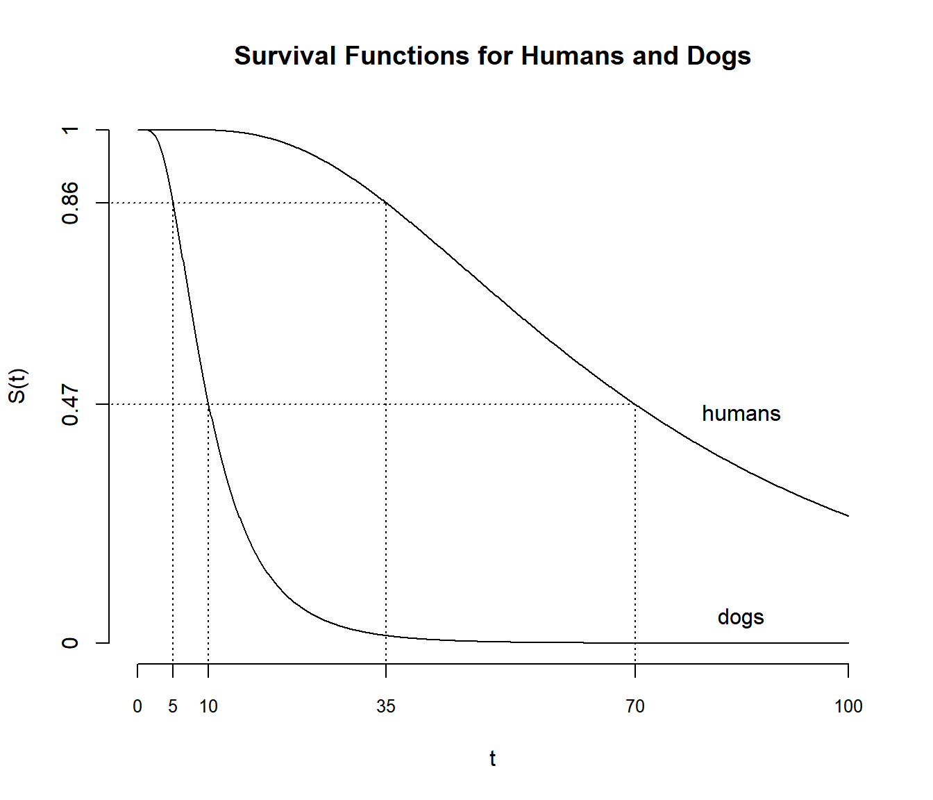
Example: Recall the AFT model for the lifespan data where the model is $$\log T_i = \beta_0 + \beta_1 x_i,$$ where $x_i$ is an indicator variable such that $x_i$ = 1 if the species is human (so $x_a$ = 1 in the above discussion), and $x_i$ = 0 if the species is dog (so $x_b$ = 0 in the above discussion). The estimate of $\beta_1$ was $\hat\beta_1$ $\approx$ 1.946 so that $e^{\hat\beta_1}$ $\approx$ 7. The “baseline” survival function is the survival function for dogs, which we can write as $S_d(t)$. The survival function for humans is then $S_h(7t)$. For example, we estimate that the probability that a dog lives for 10 or more years equals the probability that a human will live for 70 or more years because $S_d(t) = S_h(7t)$ where $t$ = 10. The survival function of a human is obtained by “stretching” the survival function of a dog by a factor of 7.

If we re-parameters the model so that $x_i$ = 1 if the species is dog, then we have that $\hat\beta_1$ $\approx$ 1/7, so that the “baseline” survival function is for humans, and we have that $S_h(t) = S_d(t/7)$. We can also say that we estimate that the probability that a human lives to be 35 or more equals the probability that a dog lives to be 5 or more because $S_d(t/7) = S_h(t)$ where $t$ = 35. The survival function of a dog is obtained by “compressing” the survival function of a human by a factor of 1/7.

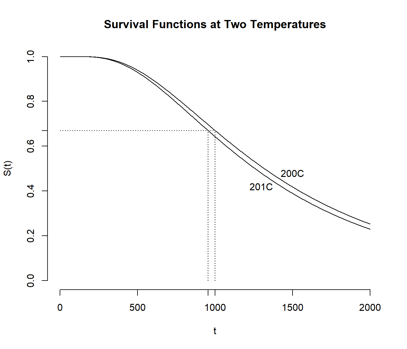
Example: Recall the AFT model for the motors data where the model is $$\log T_i = \beta_0 + \beta_1 x_i,$$ where $x_i$ is temperature. The estimate of $\beta_1$ was $\hat\beta_1$ $\approx$ -0.047 so that $e^{\hat\beta_1} \approx 0.95$. Thus $S_{x+1}(0.95t) = S_x(t)$ where the subscript of $x$ represents temperature. Increasing by one degree “compresses” the survival function by a factor of about 0.95 (i.e., 5%).

Plotting Estimated Survival Functions

Estimating and plotting survival functions is relatively easy using flexsurvreg objects. Here the summary function behaves more like predict for other model objects produced by lm, nls, and glm.

Example: The estimated survival functions for the AFT model for the lifespan data can be computed/plotted as follows.

library(trtools) # for lifespan data
m <- flexsurvreg(Surv(years) ~ species, dist = "lognormal", data = lifespan)
 
d <- data.frame(species = c("dog","human"))
d <- summary(m, newdata = d, t = seq(0, 100, by = 0.5), type = "survival", tidy = TRUE)
head(d)

  time   est   lcl   ucl species
1  0.0 1.000 1.000 1.000     dog
2  0.5 1.000 1.000 1.000     dog
3  1.0 1.000 1.000 1.000     dog
4  1.5 0.999 0.999 0.999     dog
5  2.0 0.995 0.994 0.996     dog
6  2.5 0.987 0.984 0.990     dog

tail(d)

     time   est   lcl   ucl species
397  97.5 0.261 0.240 0.282   human
398  98.0 0.258 0.238 0.280   human
399  98.5 0.256 0.235 0.277   human
400  99.0 0.253 0.232 0.274   human
401  99.5 0.250 0.230 0.271   human
402 100.0 0.248 0.227 0.268   human

p <- ggplot(d, aes(x = time, y = est)) + 
  geom_line(aes(linetype = species)) + 
  labs(x = "Time (years)", y = "S(t)", linetype = "Species") + 
  theme_minimal() + 
  theme(legend.position = "inside", legend.position.inside = c(0.8,0.8))
plot(p)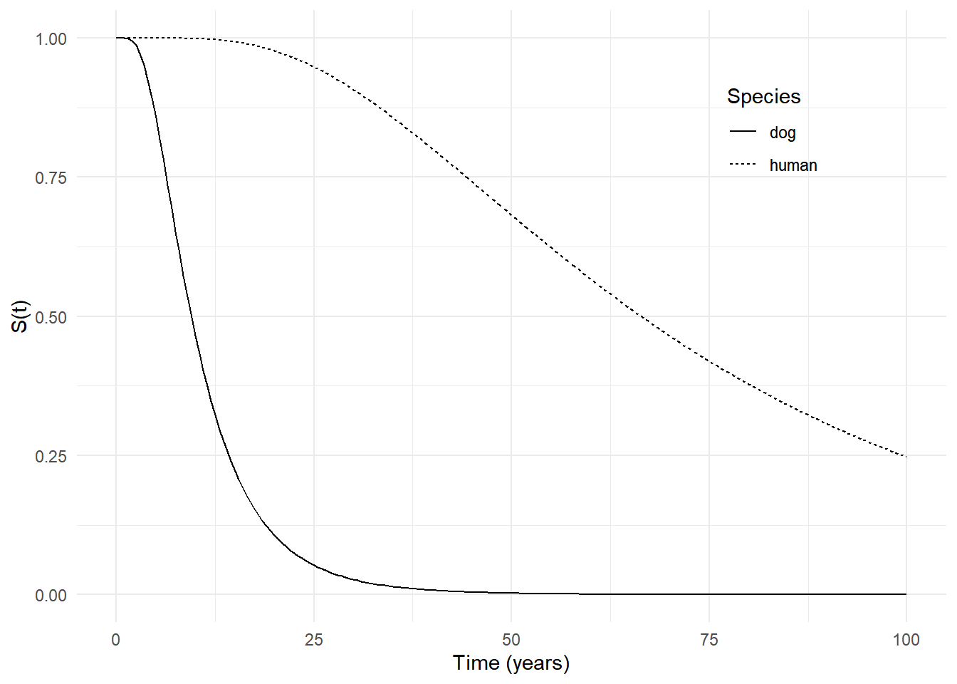

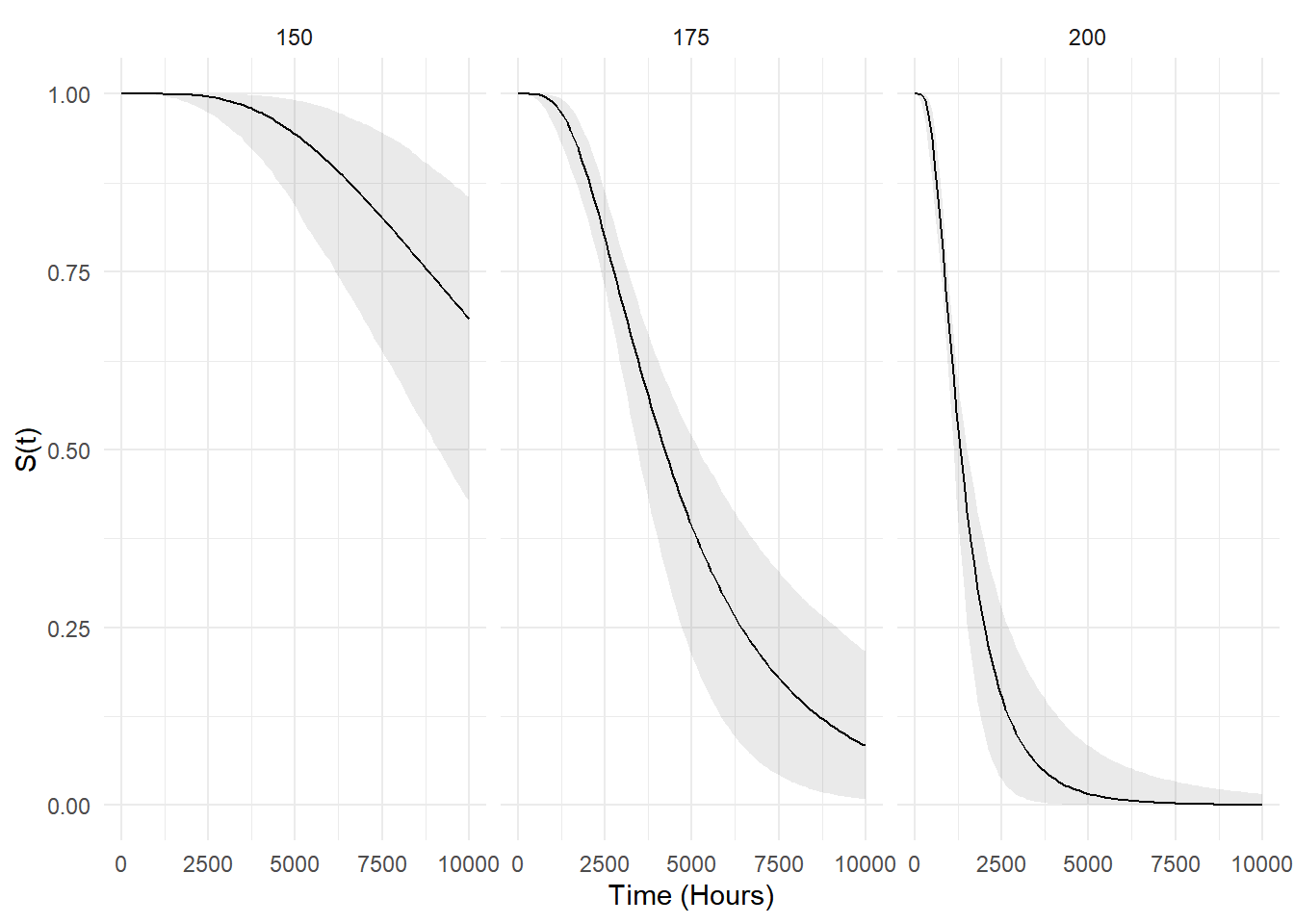
Example: Survival functions at different temperatures based on the AFT model for the motors data can be computed/plotted as follows.

library(MASS) # for motors data frame
m <- flexsurvreg(Surv(time, cens) ~ temp, dist = "lognormal", data = motors)

d <- data.frame(temp = c(150,175,200))
d <- summary(m, newdata = d, t = seq(0, 10000, length = 100), 
 type = "survival", tidy = TRUE)

p <- ggplot(d, aes(x = time, y = est, linetype = factor(temp))) + 
  geom_line() + theme_minimal() + 
  labs(x = "Time (Hours)", y = "S(t)", linetype = "Temperature (C)") 
plot(p)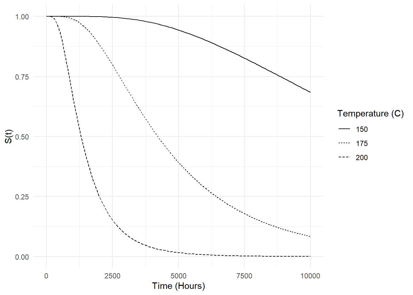

p <- ggplot(d, aes(x = time, y = est)) + 
  geom_line() + facet_wrap(~ temp, nrow = 1) + 
  geom_ribbon(aes(ymin = lcl, ymax = ucl), alpha = 0.1) +
  labs(x = "Time (Hours)", y = "S(t)") + theme_minimal()
plot(p)