Friday, February 21

You can also download a PDF copy of this lecture.

The Michaelis-Menten Model

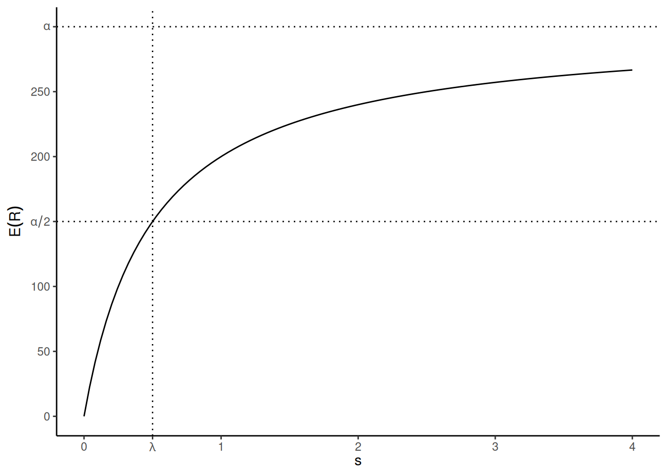
The Michaelis-Menten model is perhaps the quintessential example of an application of nonlinear regression. It is from biochemistry and concerns the relationship between the (expected) rate of an enzymatic reaction to the concentration of an enzymatic substrate (i.e., the material of the reaction). As a nonlinear regression model the Michaelis-Menten model can be written as \[ E(R) = \frac{\alpha s}{\lambda + s}, \] where $Y$ is the reaction rate and $x$ is the substrate concentration.¹

The two parameters of this model, $\alpha$ and $\lambda$, are interpretable in terms of the relationship between the expected reaction rate and substrate concentration. The $\alpha$ parameter is the maximum expected reaction rate (i.e., the upper asymptote as $s \rightarrow \infty$), and $\lambda$ is the value of $x$ at which the reaction rate is half of $\alpha$ (i.e., a “half-life” parameter) so smaller values of $\lambda$ mean that the curve is approaching $\alpha$ “faster” as $s$ increases.² Note also that if $s = 0$ then $E(R) = 0$ so the curve is constrained to have an “intercept” of zero, which makes sense in the context of enzyme kinetics. The plot below shows an example of the model where $\alpha$ = 300 and $\lambda$ = 0.5. To estimate $\alpha$ and $\lambda$ the typical method is to conduct a series of assays, varying substrate concentration and recording the reaction rate at each concentration, and then using nonlinear regression to estimate $\alpha$ and $\lambda$. In the following problems you will be using data in the data frame Puromycin. It is included with R so there is no package to load. These data are from a study that observed reaction rates at several substrate concentrations, but also for cells that were treated with puromycin (an antibiotic). Before starting you can familiarize yourself with the data by simply typing Puromycin at the console prompt (it is not a large data set).

To get started we will first ignore the experimental manipulation of treated cells with puromycin. The R code below will estimate the linear model $E(R_i) = \beta_0 + \beta_1 s_i$ using nls and plot this model with the data.

library(ggplot2)
m <- nls(rate ~ b0 + b1 * conc, start = c(b0 = 0, b1 = 0), data = Puromycin)

d <- expand.grid(conc = seq(0, 1.2, length = 100), state = c("treated","untreated"))
d$yhat <- predict(m, newdata = d)

p <- ggplot(Puromycin, aes(x = conc, y = rate)) + 
  geom_point(aes(color = state)) + geom_line(aes(y = yhat), data = d) + 
  labs(x = "Substrate Concentration (ppm)", 
    y = "Reaction Rate (counts/min/min)", color = "Cell State") + 
  theme_minimal() + 
  theme(legend.position = "inside", legend.position.inside = c(0.8,0.3))
plot(p)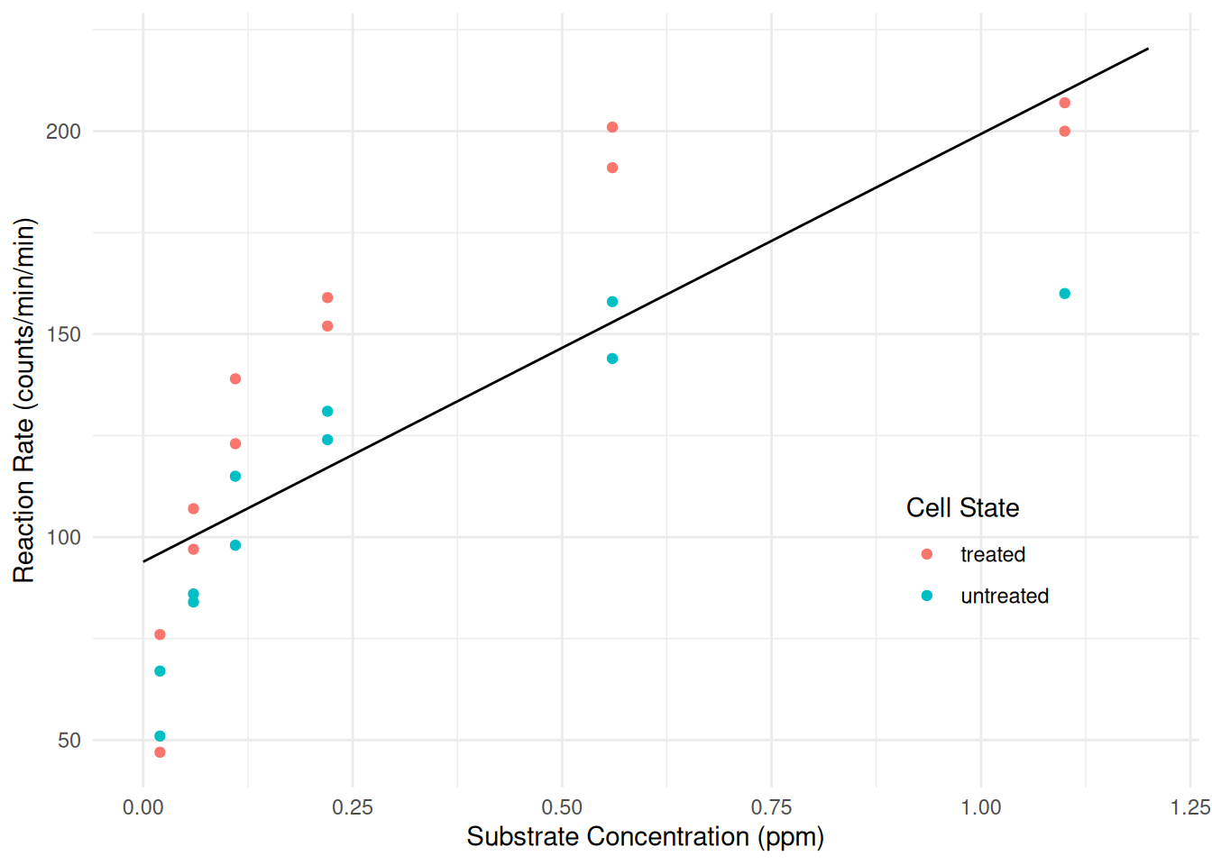

Clearly the linear model is not a good model for the data. Cut-and-paste the R code above and modify it to replace the linear model with the Michaelis-Menten model (ignoring the experimental manipulation for now). To specify starting values for $\alpha$ and $\lambda$, look at the plot of the data and try to guess their approximate values. Remember that $\alpha$ is the asymptote and $\lambda$ is the concentration at which the (expected) reaction rate is half way between zero and the asymptote.

Solution: We might estimate the nonlinear model as follows, using the figure to guess starting values for $\alpha$ and $\lambda$.

m <- nls(rate ~ alpha * conc / (lambda + conc), data = Puromycin,
  start = list(alpha = 200, lambda = 0.1))
cbind(summary(m)$coefficients, confint(m))

        Estimate Std. Error t value  Pr(>|t|)      2.5%     97.5%
alpha  190.80620    8.76458  21.770 6.835e-16 172.68402 210.97021
lambda   0.06039    0.01077   5.608 1.449e-05   0.03981   0.08881

We can plot the model as follows by “adding” to the code above.

d <- data.frame(conc = seq(0, 1.2, length = 100))
d$yhat <- predict(m, newdata = d)
p <- p + geom_line(aes(y = yhat), data = d, linetype = 2)
plot(p)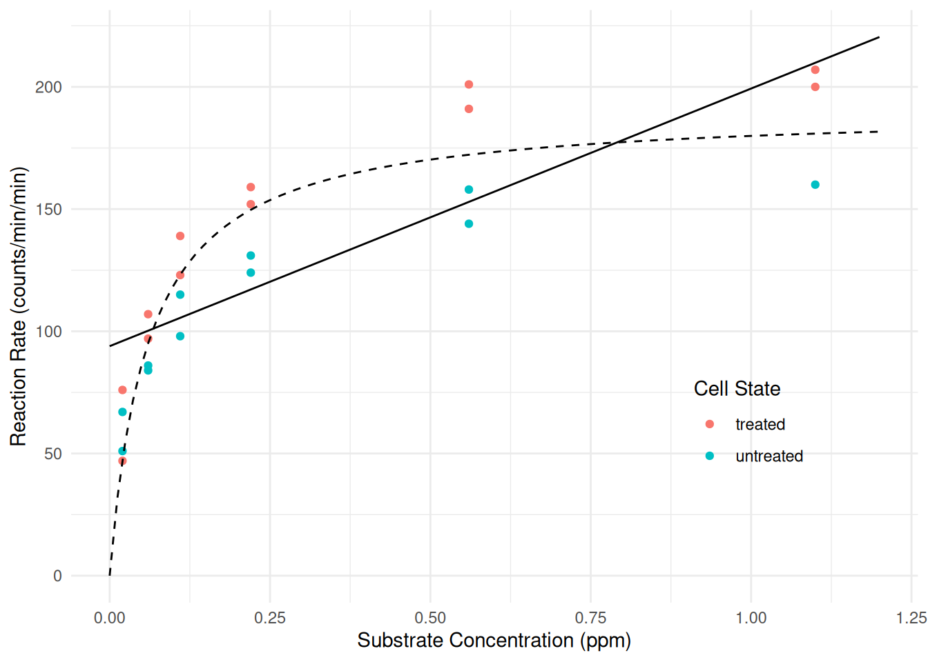

Now consider a linear model that will assume a linear relationship between reaction rate and concentration that is different for treated versus untreated cells (i.e., an “interaction” between substrate concentration and cell state).

m <- lm(rate ~ state + conc + conc:state, data = Puromycin)
cbind(summary(m)$coefficients, confint(m))

                    Estimate Std. Error t value  Pr(>|t|)  2.5 % 97.5 %
(Intercept)           103.49      10.53   9.832 6.914e-09  81.46 125.52
stateuntreated        -17.45      15.06  -1.158 2.611e-01 -48.98  14.08
conc                  110.42      20.46   5.397 3.301e-05  67.60 153.24
stateuntreated:conc   -21.08      32.69  -0.645 5.266e-01 -89.50  47.33

From summary we can see that the model can be written as \[ E(R_i) = \beta_0 + \beta_1 u_i + \beta_2 s_i + \beta_3 u_i s_i, \] where $s_i$ represents concentration (conc) and $u_i$ is an indicator variable for when the treatment (state) is “untreated” so that \[ u_i = \begin{cases} 1, & \text{if the $i$-th observation is of untreated cells}, \\ 0, & \text{otherwise}. \end{cases} \] This model can be written case-wise as \[ E(R_i) = \begin{cases} \beta_0 + \beta_2 s_i, & \text{if the $i$-th observation is of treated cells,} \\ \beta_0 + \beta_1 + (\beta_2 + \beta_3) s_i,& \text{if the $i$-th observation is of untreated cells.} \end{cases} \] We can replicate this model using the nls function by specifying an indicator variable in the model formula.

m <- nls(rate ~ b0 + b1*(state == "untreated") + 
  b2*conc + b3*(state == "untreated")*conc,
  data = Puromycin, start = list(b0 = 0, b1 = 0, b2 = 0, b3 = 0))
summary(m)$coefficients

   Estimate Std. Error t value  Pr(>|t|)
b0   103.49      10.53   9.832 6.914e-09
b1   -17.45      15.06  -1.158 2.611e-01
b2   110.42      20.46   5.397 3.301e-05
b3   -21.08      32.69  -0.645 5.266e-01

d <- expand.grid(conc = seq(0, 1.2, length = 100), state = c("treated","untreated"))
d$yhat <- predict(m, newdata = d)

p <- ggplot(Puromycin, aes(x = conc, y = rate, color = state)) + 
  geom_point() + geom_line(aes(y = yhat), data = d) + 
  labs(x = "Substrate Concentration (ppm)",
    y = "Reaction Rate (counts/min/min)", color = "Cell State") + 
  theme_minimal() + 
  theme(legend.position = "inside", legend.position.inside = c(0.8,0.3))
plot(p)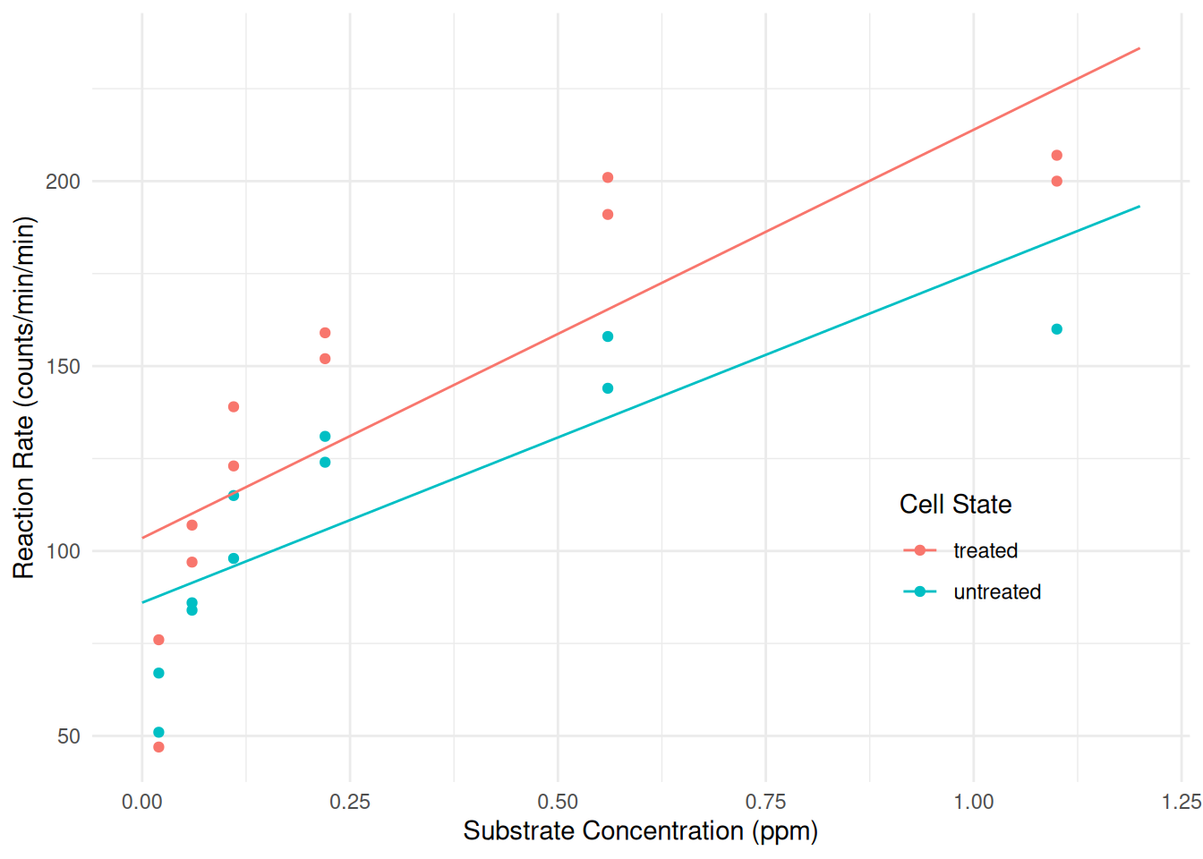

Since there are only two levels of state we could also use the ifelse function to produce the same results as using the indicator variable.

m <- nls(rate ~ ifelse(state == "treated", b0 + b2*conc, b0 + b1 + (b2 + b3)*conc),
  data = Puromycin, start = list(b0 = 0, b1 = 0, b2 = 0, b3 = 0))
summary(m)$coefficients

   Estimate Std. Error t value  Pr(>|t|)
b0   103.49      10.53   9.832 6.914e-09
b1   -17.45      15.06  -1.158 2.611e-01
b2   110.42      20.46   5.397 3.301e-05
b3   -21.08      32.69  -0.645 5.266e-01

We can also use the case_when function from the dplyr package.

library(dplyr)
m <- nls(rate ~ case_when(
  state == "treated" ~ b0 + b2*conc, 
  state == "untreated" ~ b0 + b1 + (b2 + b3)*conc,
), data = Puromycin, start = list(b0 = 0, b1 = 0, b2 = 0, b3 = 0))
summary(m)$coefficients

   Estimate Std. Error t value  Pr(>|t|)
b0   103.49      10.53   9.832 6.914e-09
b1   -17.45      15.06  -1.158 2.611e-01
b2   110.42      20.46   5.397 3.301e-05
b3   -21.08      32.69  -0.645 5.266e-01

Obviously this is a poor model for the Puromycin data since expected reaction rate does not appear to be a linear function of substrate concentration. Instead we would like to have a model where there the Michaelis-Menten model describes the relationship between the expected reaction rate and substrate concentration, but differently for each state so that the $\alpha$ and $\lambda$ parameters can depend on the state. Estimate this model using the nls function, noting that there are many different ways that this model could be parameterized. Plot the model as well with the raw data.

Solution: Here is one way we might specify such a model.

m1 <- nls(rate ~ ifelse(state == "treated", alphat * conc / (lambdat + conc),
  alphau * conc / (lambdau + conc)), data = Puromycin,
  start = list(alphat = 200, lambdat = 0.1, alphau = 200, lambdau = 0.1))
cbind(summary(m1)$coefficients, confint(m1))

         Estimate Std. Error t value  Pr(>|t|)      2.5%     97.5%
alphat  212.68373   6.608094  32.185 4.876e-18 198.88883 227.45563
lambdat   0.06412   0.007877   8.141 1.293e-07   0.04856   0.08354
alphau  160.28001   6.896012  23.242 2.041e-15 145.85285 176.28021
lambdau   0.04771   0.008281   5.761 1.496e-05   0.03159   0.06966

The case_when function could also be used here.

m1 <- nls(rate ~ case_when(
  state == "treated"   ~ alphat * conc / (lambdat + conc),
  state == "untreated" ~ alphau * conc / (lambdau + conc)), data = Puromycin,
  start = list(alphat = 200, lambdat = 0.1, alphau = 200, lambdau = 0.1))
cbind(summary(m1)$coefficients, confint(m1))

         Estimate Std. Error t value  Pr(>|t|)      2.5%     97.5%
alphat  212.68373   6.608094  32.185 4.876e-18 198.88883 227.45563
lambdat   0.06412   0.007877   8.141 1.293e-07   0.04856   0.08354
alphau  160.28001   6.896012  23.242 2.041e-15 145.85285 176.28021
lambdau   0.04771   0.008281   5.761 1.496e-05   0.03159   0.06966

This model can be written as \[ E(Y_i) = \begin{cases} \alpha_t s_i/(\lambda_t + s_i), & \text{if the $i$-th observation is of treated cells}, \\ \alpha_u s_i/(\lambda_u + s_i), & \text{if the $i$-th observation is of untreated cells}. \end{cases} \] An alternative paramterization that includes a parameter for the “effect” of treating the cells is \[ E(Y_i) = \begin{cases} (\alpha + \delta_{\alpha})s_i/(\lambda + \delta_{\lambda} + s_i), & \text{if the $i$-th observation is of treated cells}, \\ \alpha s_i/(\lambda + s_i), & \text{if the $i$-th observation is of untreated cells}. \end{cases} \] This is slightly different from the model shown in lecture, because here the “baseline” parameters $\alpha$ and $\lambda$ are for the untreated cells. We can see a relationship between the parameters in the two models: $\alpha = \alpha_u$, $\lambda = \lambda_u$, $\delta_{\alpha} = \alpha_t - \alpha_u$ and $\delta_{\lambda} = \lambda_t - \lambda_u$. This latter model can be estimated as follows.

m2 <- nls(rate ~ ifelse(state == "treated",
  (alpha + deltaa) * conc / (lambda + deltal + conc),
  alpha * conc / (lambda + conc)), data = Puromycin,
  start = list(alpha = 200, lambda = 0.1, deltaa = 0, deltal = 0))
cbind(summary(m2)$coefficients, confint(m2))

        Estimate Std. Error t value  Pr(>|t|)      2.5%     97.5%
alpha  160.28001   6.896011  23.242 2.041e-15 145.85285 176.28021
lambda   0.04771   0.008281   5.761 1.496e-05   0.03159   0.06966
deltaa  52.40373   9.551014   5.487 2.713e-05  31.33677  73.09295
deltal   0.01641   0.011429   1.436 1.672e-01  -0.01043   0.04187

There are several other ways we might parameterize the model and specify it in nls. But for plotting purposes the parameterization does not matter.

d <- expand.grid(conc = seq(0, 1.2, length = 100), state = c("treated","untreated"))
d$yhat <- predict(m1, newdata = d)

p <- ggplot(Puromycin, aes(x = conc, y = rate, color = state)) +
  geom_point() + geom_line(aes(y = yhat), data = d) +
  labs(x = "Substrate Concentration (ppm)",
    y = "Reaction Rate (counts/min/min)") +
  labs(color = "Cell State") +
  theme_minimal() + 
  theme(legend.position = "inside", legend.position.inside = c(0.8,0.3))
plot(p)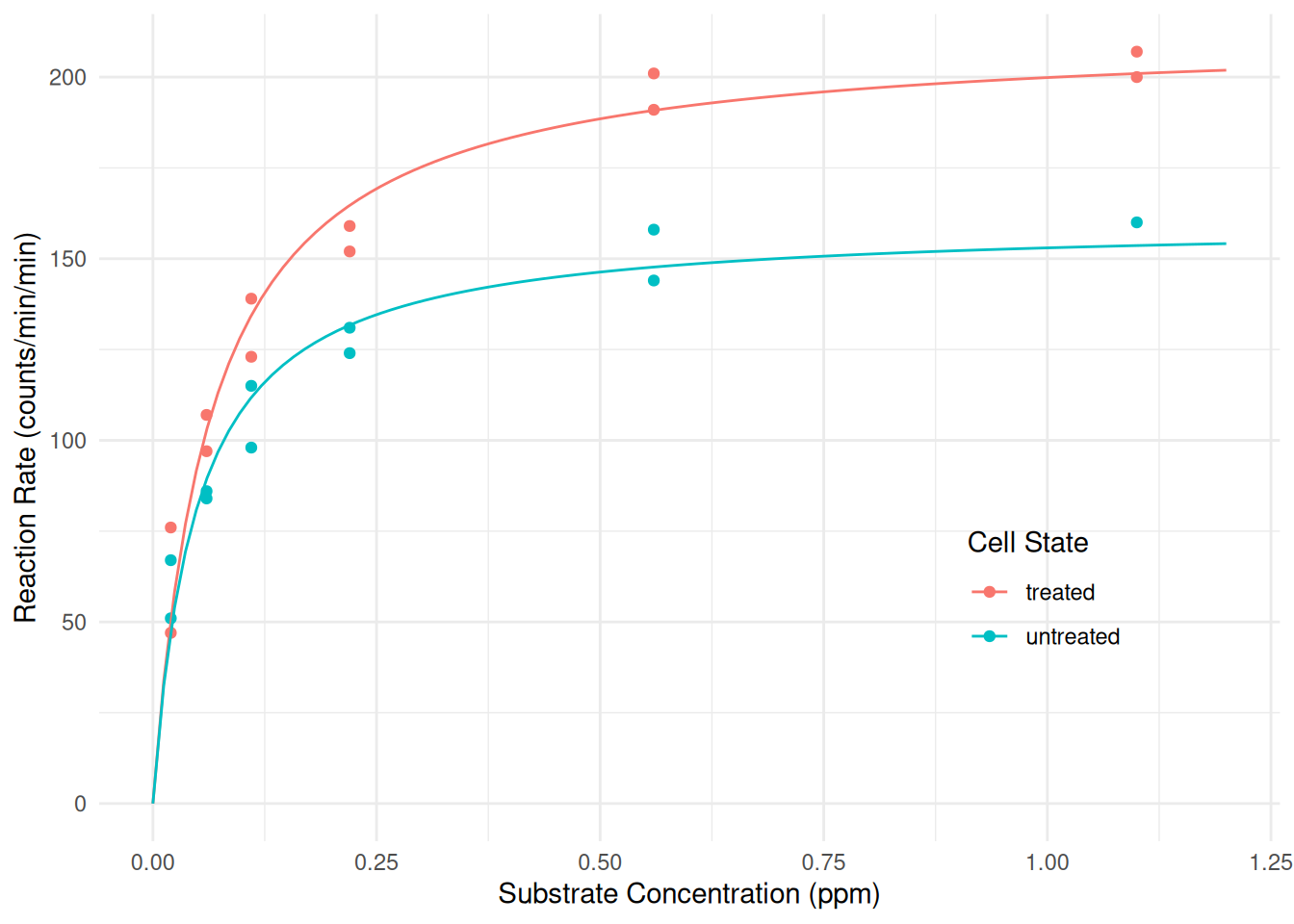

There are several potentially useful inferences we might make here. One is the values of the two parameters for the Michaelis-Menten model for each state. Another is the difference in the parameters between states. Depending on how the model was parameterized in the previous question, some of these could be found simply by using summary and confint, while others might require using lincon unless the model is reparameterized. Produce estimates, standard errors, and confidence intervals for the six quantities described above.

Solution: First consider inferences for the two parameters of the Michaelis-Menten model for each treatment condition. These are the parameters of the first parameterization used above.
```
cbind(summary(m1)$coefficients, confint(m1))
```
```
         Estimate Std. Error t value  Pr(>|t|)      2.5%     97.5%
alphat  212.68373   6.608094  32.185 4.876e-18 198.88883 227.45563
lambdat   0.06412   0.007877   8.141 1.293e-07   0.04856   0.08354
alphau  160.28001   6.896012  23.242 2.041e-15 145.85285 176.28021
lambdau   0.04771   0.008281   5.761 1.496e-05   0.03159   0.06966
```
If we were using the second parameterization, we could obtain estimates of the parameters from the untreated cells from summary and confint, but would have to use something like lincon to to estimate a function of the model parameters. Recall the relationships between the parameters in the two models: $\alpha = \alpha_u$, $\lambda = \lambda_u$, $\delta_{\alpha} = \alpha_t - \alpha_u$ and $\delta_{\lambda} = \lambda_t - \lambda_u$. Thus $\alpha_t = \alpha + \delta_{\alpha}$ and $\lambda_t = \lambda + \delta_{\lambda}$.
```
library(trtools)
cbind(summary(m2)$coefficients, confint(m2))
```
```
        Estimate Std. Error t value  Pr(>|t|)      2.5%     97.5%
alpha  160.28001   6.896011  23.242 2.041e-15 145.85285 176.28021
lambda   0.04771   0.008281   5.761 1.496e-05   0.03159   0.06966
deltaa  52.40373   9.551014   5.487 2.713e-05  31.33677  73.09295
deltal   0.01641   0.011429   1.436 1.672e-01  -0.01043   0.04187
```
```
lincon(m2, a = c(1, 0, 1, 0)) # lambdat  
```
```
            estimate    se lower upper tvalue df    pvalue
(1,0,1,0),0    212.7 6.608 198.9 226.5  32.19 19 4.876e-18
```
```
lincon(m2, a = c(0, 1, 0, 1)) # lambdat 
```
```
            estimate       se   lower   upper tvalue df    pvalue
(0,1,0,1),0  0.06412 0.007877 0.04763 0.08061  8.141 19 1.293e-07
```
Now if we want to estimate the difference in the parameters of the Michaelis-Menten model between the treated and untreated states, we could get that from the second parameterization because those differences are $\delta_{\alpha}$ and $\delta_{\lambda}$.
```
cbind(summary(m2)$coefficients, confint(m2))
```
```
        Estimate Std. Error t value  Pr(>|t|)      2.5%     97.5%
alpha  160.28001   6.896011  23.242 2.041e-15 145.85285 176.28021
lambda   0.04771   0.008281   5.761 1.496e-05   0.03159   0.06966
deltaa  52.40373   9.551014   5.487 2.713e-05  31.33677  73.09295
deltal   0.01641   0.011429   1.436 1.672e-01  -0.01043   0.04187
```
But if we were using the first parameterization we would again need to use something like lincon since $\delta_{\alpha} = \alpha_t - \alpha_u$ and $\delta_{\lambda} = \lambda_t - \lambda_u$.
```
lincon(m1, a = c(1,0,-1,0)) # delta_alpha
```
```
             estimate    se lower upper tvalue df    pvalue
(1,0,-1,0),0     52.4 9.551 32.41 72.39  5.487 19 2.713e-05
```
```
lincon(m1, a = c(0,1,0,-1)) # delta_lambda
```
```
             estimate      se     lower   upper tvalue df pvalue
(0,1,0,-1),0  0.01641 0.01143 -0.007508 0.04033  1.436 19 0.1672
```
Note that when estimating the same quantity we obtain the same estimates and standard errors from either parameterization from summary and lincon. The confidence intervals, however, are slightly different because confint and lincon use different methods of obtaining approximate confidence intervals.

Heteroscedasticity in the Daphnia Data

The data frame daphniastrat from the trtools package features data from a survey of water fleas where the number of water fleas were counted in one liter samples of water taken from three different layers of a lake.

library(trtools) # for daphniastrat
library(ggplot2) 
p <- ggplot(daphniastrat, aes(x = layer, y = count)) + 
  geom_dotplot(binaxis = "y", binwidth = 1, stackdir = "center") + 
  labs(x = "Layer", y = "Number of Daphnia") + theme_minimal()
plot(p)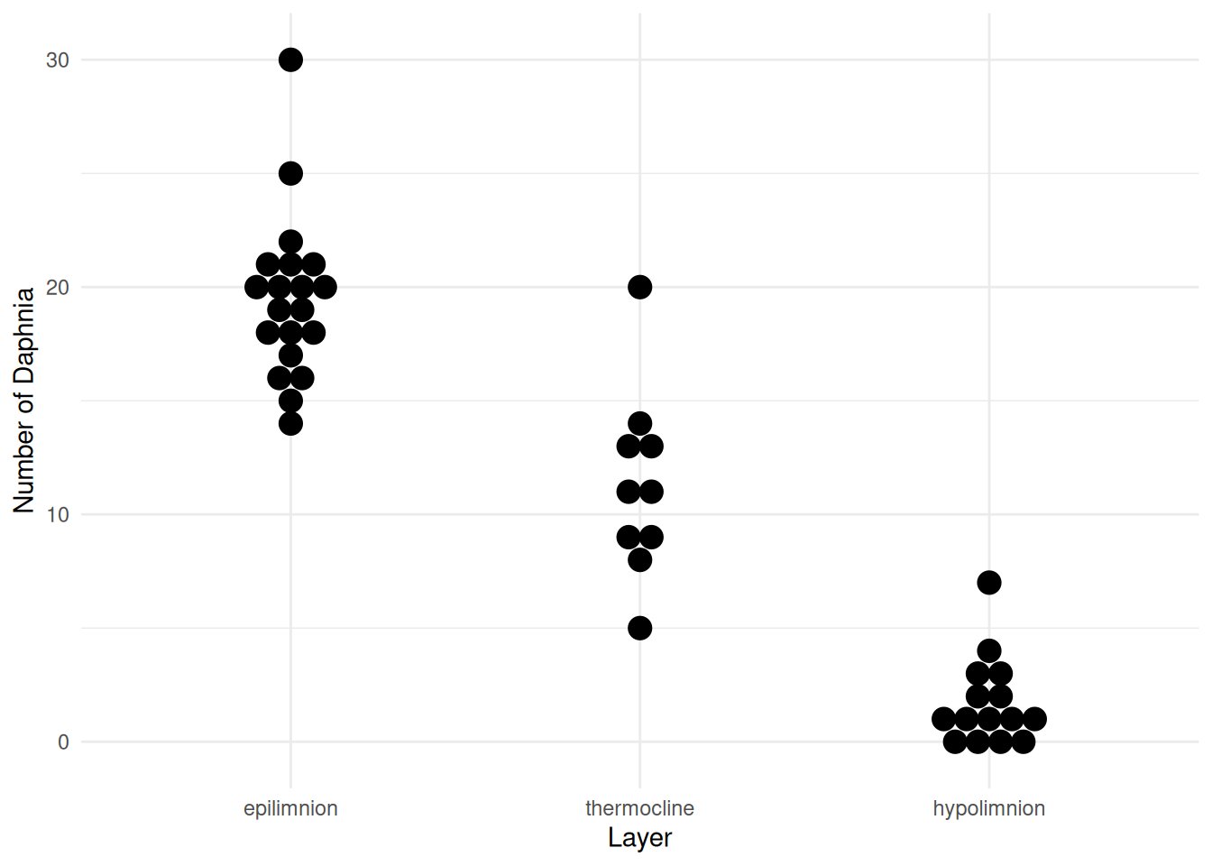

We used the following linear model for these data.

m <- lm(count ~ layer, data = daphniastrat)
summary(m)$coefficients

                 Estimate Std. Error t value  Pr(>|t|)
(Intercept)         19.50     0.7271  26.820 4.727e-28
layerthermocline    -8.20     1.2593  -6.512 7.293e-08
layerhypolimnion   -17.77     1.1106 -15.997 1.784e-19

But heteroscedasticity is evident in the plot of the raw data above and also in a plot of the studentized residuals.

daphniastrat$yhat <- predict(m)
daphniastrat$rest <- rstudent(m)
p <- ggplot(daphniastrat, aes(x = yhat, y = rest, color = layer)) + 
  geom_count() + theme_minimal() + 
  labs(x = "Predicted Value", y = "Studentized Residual", color = "Layer")
plot(p)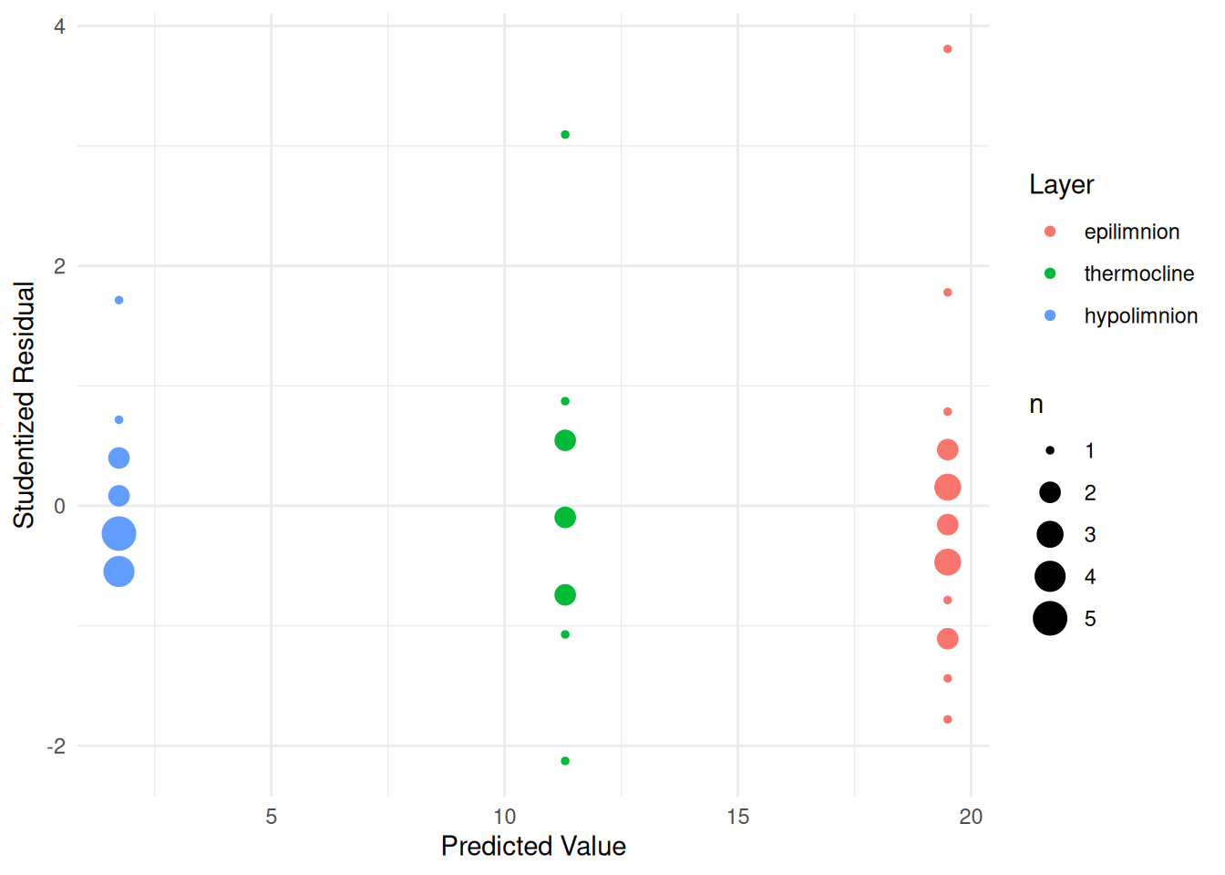

Note that geom_count is a variant of geom_point that makes the point size proportional to the number of points at a particular position, which is useful here.

Heteroscedasticty is quite common when the response variable is a count. Typically the variance of the counts increases with the expected count. Here we will consider a couple of ways of dealing with this heteroscedasticty.

We might assume that the variance varies by layer with the expected count, so that \[ \text{Var}(Y_i) = \begin{cases} \sigma_e^2, & \text{if the $i$-th observation is from the epilimnion layer}, \\ \sigma_t^2, & \text{if the $i$-th observation is from the thermocline layer}, \\ \sigma_h^2, & \text{if the $i$-th observation is from the hypolimnion layer}. \end{cases} \] If so, then our weights should be specified such that \[ w_i \propto \begin{cases} 1/\sigma_e^2, & \text{if the $i$-th observation is from the epilimnion layer}, \\ 1/\sigma_t^2, & \text{if the $i$-th observation is from the thermocline layer}, \\ 1/\sigma_h^2, & \text{if the $i$-th observation is from the hypolimnion layer}. \end{cases} \] We do not know $\sigma_e^2$, $\sigma_t^2$, and $\sigma_h^2$, but they could be estimated using the sample variances $s_e^2$, $s_t^2$, and $s_h^2$, respectively, which we can easily compute since we have multiple observations from each layer. Estimate the model using weighted least squares with weights computed as described above. The sample variances can be computed and used to add weights to the data frame using functions from the dplyr package as demonstrated with the CancerSurvival data in lecture.

Solution: First we compute the weights using functions from the dplyr package.
```
library(dplyr)
daphniastrat <- daphniastrat %>% group_by(layer) %>% mutate(w = 1 / var(count))
```
Then we estimate the model using weighted least squares.
```
m <- lm(count ~ layer, data = daphniastrat, weights = w)
summary(m)$coefficients
```
```
                 Estimate Std. Error t value  Pr(>|t|)
(Intercept)         19.50     0.7997  24.385 2.035e-26
layerthermocline    -8.20     1.5190  -5.398 2.896e-06
layerhypolimnion   -17.77     0.9392 -18.918 3.617e-22
```

Assuming again that the variance of the counts vary by layer so that \[ \text{Var}(Y_i) = \begin{cases} \sigma_e^2, & \text{if the $i$-th observation is from the epilimnion layer}, \\ \sigma_t^2, & \text{if the $i$-th observation is from the thermocline layer}, \\ \sigma_h^2, & \text{if the $i$-th observation is from the hypolimnion layer}, \end{cases} \] another approach would be to use a parametric model that estimates the usual parameters of the regression model (i.e., $\beta_0$, $\beta_1$, and $\beta_3$) and the three variances above simultaneously. Do this using the gls function from the nlme package as demonstrated in lecture.

Solution: Here is how we would estimate this model.

library(nlme) # for gls function
m <- gls(count ~ layer, data = daphniastrat,
  weights = varIdent(form = ~ 1 | layer), method = "ML")
summary(m)

Generalized least squares fit by maximum likelihood
  Model: count ~ layer 
  Data: daphniastrat 
    AIC   BIC logLik
  235.1 245.9 -111.5

Variance function:
 Structure: Different standard deviations per stratum
 Formula: ~1 | layer 
 Parameter estimates:
 epilimnion thermocline hypolimnion 
     1.0000      1.1115      0.5286 

Coefficients:
                  Value Std.Error t-value p-value
(Intercept)       19.50    0.8068  24.170       0
layerthermocline  -8.20    1.5030  -5.456       0
layerhypolimnion -17.77    0.9452 -18.796       0

 Correlation: 
                 (Intr) lyrthr
layerthermocline -0.537       
layerhypolimnion -0.854  0.458

Standardized residuals:
    Min      Q1     Med      Q3     Max 
-1.6261 -0.5937 -0.1434  0.4303  3.0123 

Residual standard error: 3.486 
Degrees of freedom: 45 total; 42 residual

The model above was estimated using maximum likelihood (ML). But another method is to use what is called restricted maximum likelihood (REML) which is the default method. It is interesting to note that for this model, this REML effectively equivalent to the approach used in the previous problem.

library(nlme) # for gls function
m <- gls(count ~ layer, data = daphniastrat,
  weights = varIdent(form = ~ 1 | layer), method = "ML")
summary(m)

Generalized least squares fit by maximum likelihood
  Model: count ~ layer 
  Data: daphniastrat 
    AIC   BIC logLik
  235.1 245.9 -111.5

Variance function:
 Structure: Different standard deviations per stratum
 Formula: ~1 | layer 
 Parameter estimates:
 epilimnion thermocline hypolimnion 
     1.0000      1.1115      0.5286 

Coefficients:
                  Value Std.Error t-value p-value
(Intercept)       19.50    0.8068  24.170       0
layerthermocline  -8.20    1.5030  -5.456       0
layerhypolimnion -17.77    0.9452 -18.796       0

 Correlation: 
                 (Intr) lyrthr
layerthermocline -0.537       
layerhypolimnion -0.854  0.458

Standardized residuals:
    Min      Q1     Med      Q3     Max 
-1.6261 -0.5937 -0.1434  0.4303  3.0123 

Residual standard error: 3.486 
Degrees of freedom: 45 total; 42 residual

We will discuss maximum likelihood and perhaps restricted maximum likelihood later in the course.

With counts it is often assumed that the variance is proportional to the expected response — i.e., $\text{Var}(Y_i) \propto E(Y_i)$. Assuming that is true here, estimate the model using iteratively weighted least squares as was demonstrated in lecture.

Solution: We can program the iteratively weighted least squares algorithm as follows.

daphniastrat$w <- 1
for (i in 1:5) {
  m <- lm(count ~ layer, data = daphniastrat, weights = w)
  daphniastrat$w <- 1 / predict(m)
}
summary(m)


Call:
lm(formula = count ~ layer, data = daphniastrat, weights = w)

Weighted Residuals:
   Min     1Q Median     3Q    Max 
-1.874 -0.684 -0.113  0.340  4.000 

Coefficients:
                 Estimate Std. Error t value Pr(>|t|)    
(Intercept)         19.50       1.13   17.24  < 2e-16 ***
layerthermocline    -8.20       1.66   -4.93  1.3e-05 ***
layerhypolimnion   -17.77       1.20  -14.85  < 2e-16 ***
---
Signif. codes:  0 '***' 0.001 '**' 0.01 '*' 0.05 '.' 0.1 ' ' 1

Residual standard error: 1.15 on 42 degrees of freedom
Multiple R-squared:  0.86,  Adjusted R-squared:  0.853 
F-statistic:  128 on 2 and 42 DF,  p-value: <2e-16

For this particular model the algorithm only needs to go through one iteration to compute the weights. This is because the predicted values do not depend on the weights in this particular model.

See the Wikipedia entry on Michaelis-Menten for details if you are interested. A related model is the Beverton-Holt population dynamics model that is frequently used in fisheries research.↩︎
The interpretation of $\alpha$ can be seen by taking the limit of $\alpha s/(\lambda + s)$ as $s \rightarrow \infty$, and the interpretation of $\lambda$ can be shown by replacing $s$ with $\lambda$ in $\alpha s/(\lambda + s)$ which gives $\alpha/2$.↩︎