Wednesday, February 5

You can also download a PDF copy of this lecture.

Linear Versus Nonlinear Models

A nonlinear regression model is any model that cannot be written as \[ E(Y_i) = \beta_0 + \beta_1 x_{i1} + \beta_2 x_{i2} + \cdots + \beta_k x_{ik}, \] such that \(x_{i1}, x_{i2}, \dots, x_{ik}\) do not depend on any unknown parameters. A linear model must be linear in the parameters.

Example: Let’s consider an exponential model for the ToothGrowth data, ignoring supplement type for now, such that \[ E(Y_i) = \beta_0 + \beta_12^{-d_i/h} \] where \(Y_i\) is length and \(d_i\) is dose. If \(h\) is specified (say \(h\) = 1) we have a linear model that we can write as \[ E(Y_i) = \beta_0 + \beta_1x_i, \] where \(x_i = 2^{-d_i/1}\). We can estimate this model in the usual way using lm.

m <- lm(len ~ I(2^(-dose/1)), data = ToothGrowth)
summary(m)$coefficients

               Estimate Std. Error t value  Pr(>|t|)
(Intercept)       35.14      1.555   22.60 1.942e-30
I(2^(-dose/1))   -33.61      2.988  -11.25 3.303e-16

But suppose we want to treat \(h\) as an unknown parameter to be estimated like \(\beta_0\) and \(\beta_1\)? This would not be a linear model. We can write the model as \[ E(Y_i) = \beta_0 + \beta_1x_i, \] where \(x_i = 2^{d_i/h}\), but now \(x_i\) depends on an unknown parameter (\(h\)) and so the model is not linear in the parameters and thus not a linear model.

Nonlinear Regression

The nls function can be used to estimate a nonlinear regression model (the nls stands for “nonlinear least squares”). But its arguments are a little different from lm.

1. The model must be written mathematically rather than symbolically. And this requires that we know the correct operators/functions in R corresponding to the desired mathematical operators/functions.

2. The starting values of the parameter estimates must be provided. This does two things: it identifies what parts of the model formula are parameters, and it provides initial values for an algorithm to use to solve the least squares optimization problem.

Example: First we will replicate the results for the linear model where \(h\) is known/specified, but now using nls.

m <- nls(len ~ beta0 + beta1*2^(-dose/1), data = ToothGrowth,
  start = list(beta0 = 0, beta1 = 0))
summary(m)$coefficients

      Estimate Std. Error t value  Pr(>|t|)
beta0    35.14      1.555   22.60 1.942e-30
beta1   -33.61      2.988  -11.25 3.303e-16

Note the starting values. For a linear model we (usually) do not need to provide good starting values so zeros work just fine. Now consider a nonlinear model where \(h\) is also an unknown parameter.

m <- nls(len ~ beta0 + beta1*2^(-dose/h), data = ToothGrowth,
  start = list(beta0 = 32, beta1 = -33, h = 1))
summary(m)$coefficients

      Estimate Std. Error t value  Pr(>|t|)
beta0  27.9366     2.1482  13.005 1.062e-18
beta1 -36.6251     6.1143  -5.990 1.493e-07
h       0.4632     0.1459   3.174 2.422e-03

Specifying “good” starting values is important. What if we don’t provide good starting values?

m <- nls(len ~ beta0 + beta1*2^(-dose/h), data = ToothGrowth,
  start = list(beta0 = 0, beta1 = 0, h = 1))

Error in nlsModel(formula, mf, start, wts, scaleOffset = scOff, nDcentral = nDcntr): singular gradient matrix at initial parameter estimates

How do we find good starting values? One approach is to use an approximate model like we did here that is linear. Another approach is to “eyeball” the estimates from a plot.

We can plot the model in the usual way.

d <- expand.grid(dose = seq(0, 4, length = 100))
d$yhat <- predict(m, newdata = d)

p <- ggplot(ToothGrowth, aes(x = dose, y = len)) + 
  geom_point(aes(color = supp), alpha = 0.5) + 
  geom_line(aes(y = yhat), data = d) + 
  labs(x = "Dose (mg/day)", y = "Odontoblast Length", 
    color = "Supplement Type") + 
  theme_minimal() + 
  theme(legend.position = "inside", legend.position.inside = c(0.8,0.2))
plot(p)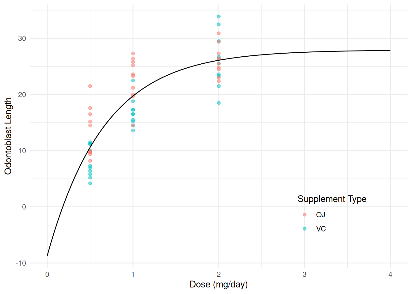

We can add some annotation if desired to highlight the interesting quantities.

summary(m)$coefficients

      Estimate Std. Error t value  Pr(>|t|)
beta0  27.9366     2.1482  13.005 1.062e-18
beta1 -36.6251     6.1143  -5.990 1.493e-07
h       0.4632     0.1459   3.174 2.422e-03

p <- p + geom_hline(yintercept = 27.94, linetype = 3) # asymptote (b0)
p <- p + geom_hline(yintercept = 27.94 - 36.63, linetype = 3) # intercept (b0 + b1)
p <- p + geom_hline(yintercept = 27.94 - 36.63/2, linetype = 3) # half-way (b0 + b1/2)
p <- p + geom_vline(xintercept = 0.46, linetype = 3) # half-life (h)
plot(p)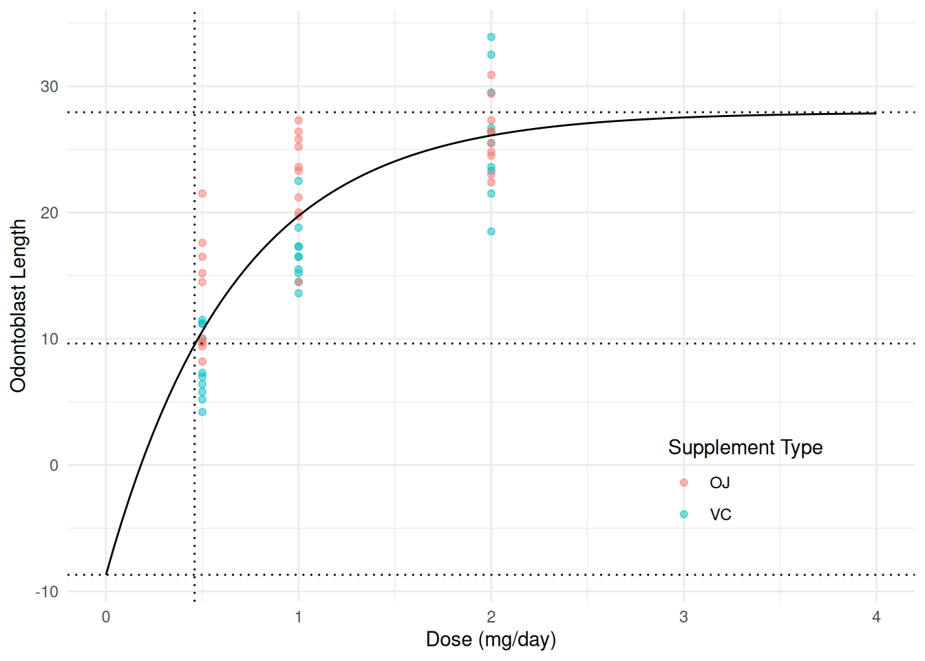

Recall that the “intercept” is \(\beta_0 + \beta_1\). We can make inferences concerning this quantity using lincon.

m <- nls(len ~ beta0 + beta1*2^(-dose/h), data = ToothGrowth, 
  start = list(beta0 = 32, beta1 = -33, h = 0.75))
lincon(m, a = c(1,1,0)) # 1*b1 + 1*b2 + 0*h = b1 + b2

          estimate    se  lower upper tvalue df pvalue
(1,1,0),0   -8.688 7.562 -23.83 6.455 -1.149 57 0.2554

Does this make sense?

We can also replicate the estimates of the asymptote (\(\beta_0\)) and half-life (\(h\)) parameters using lincon.

cbind(summary(m)$coefficients, confint(m))

      Estimate Std. Error t value  Pr(>|t|)     2.5%   97.5%
beta0  27.9366     2.1482  13.005 1.062e-18  24.7232  37.229
beta1 -36.6251     6.1143  -5.990 1.493e-07 -57.3146 -28.105
h       0.4632     0.1459   3.174 2.422e-03   0.2647   1.135

lincon(m, c(1,0,0)) # asymptote (beta0)

          estimate    se lower upper tvalue df    pvalue
(1,0,0),0    27.94 2.148 23.63 32.24     13 57 1.062e-18

lincon(m, c(0,0,1)) # half-life (h)

          estimate     se lower  upper tvalue df   pvalue
(0,0,1),0   0.4632 0.1459 0.171 0.7554  3.174 57 0.002422

Note the difference in the confidence intervals (particularly for \(h\)). Here confint and lincon using different kinds of confidence intervals: confint uses “profile-likelihood” intervals and lincon uses “Wald” intervals. We will discuss profile-likelihood confidence intervals later, but note here that typically they are more accurate.

The emmeans and contrast functions cannot (yet) be applied to a nls object. We must rely on something like lincon or clever parameterization (see below).

Now consider the model \[ E(Y_i) = \begin{cases} \beta_0 + \beta_12^{-x_i/h_{\text{OJ}}}, & \text{if the supplement type is OJ}, \\ \beta_0 + \beta_12^{-x_i/h_{\text{VC}}}, & \text{if the supplement type is VC}, \end{cases} \] where \(x_i\) is dose. There are several ways we can handle case-wise models with nls: indicator variables, the ifelse function, and the case_when function.

1. We could write the model as \[ E(Y_i) = \beta_0 + \beta_12^{-x_i/(o_ih_{\text{OJ}} + v_ih_{\text{VC}})}, \] where \(o_i\) and \(v_i\) are indicator variables for the OJ and VC supplement types, respectively. In R we can program these indicator variables as supp == "OJ" and supp == "VC", respectively. These will return TRUE or FALSE, but will be interpreted as 1 or 0, respectively, if used in a calculation. Here is how we can write this model in nls.

   m <- nls(len ~ b0 + b1*2^(-dose/((supp == "OJ")*hoj + (supp == "VC")*hvc)),
     data = ToothGrowth, start = c(b0 = 28, b1 = -37, hoj = 0.46, hvc = 0.46))   
   summary(m)$coefficients

       Estimate Std. Error t value  Pr(>|t|)
   b0   27.5018    1.39516  19.712 7.258e-27
   b1  -39.5856    5.47238  -7.234 1.422e-09
   hoj   0.3382    0.06978   4.846 1.036e-05
   hvc   0.5001    0.11208   4.462 3.963e-05

   We could actually get away with one indicator variable if we are a little clever (and we are).

   m <- nls(len ~ b0 + b1*2^(-dose/((supp == "OJ")*hoj + (1 - (supp == "OJ"))*hvc)),
     data = ToothGrowth, start = c(b0 = 28, b1 = -37, hoj = 0.46, hvc = 0.46))
   summary(m)$coefficients

       Estimate Std. Error t value  Pr(>|t|)
   b0   27.5018    1.39516  19.712 7.258e-27
   b1  -39.5856    5.47238  -7.234 1.422e-09
   hoj   0.3382    0.06978   4.846 1.036e-05
   hvc   0.5001    0.11208   4.462 3.963e-05

   Here is a plot of the model with the data.

   d <- expand.grid(dose = seq(0, 4, length = 100), supp = c("OJ","VC"))
   d$yhat <- predict(m, newdata = d)
   
   p <- ggplot(ToothGrowth, aes(x = dose, y = len, color = supp)) +
     geom_point(alpha = 0.5) + 
     geom_line(aes(y = yhat), data = d) + 
     labs(x = "Dose (mg/day)", y = "Odontoblast Length", 
       color = "Supplement Type") + 
     theme_minimal() + 
     theme(legend.position = "inside", legend.position.inside = c(0.8,0.2))
   plot(p)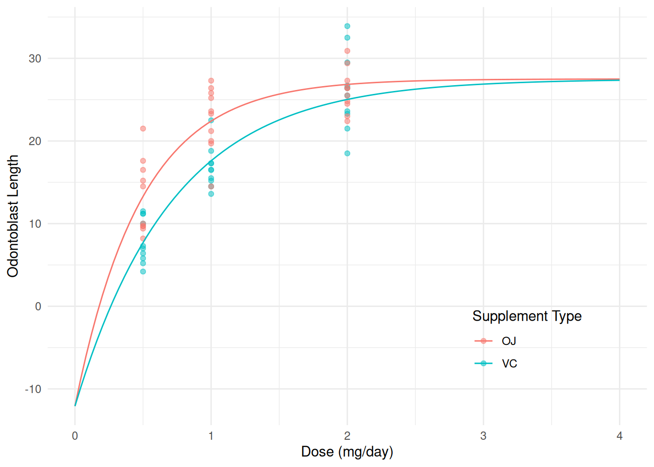

   

2. When there are only two cases it can be convenient to use ifelse.

   m <- nls(len ~ b0 + b1*2^(-dose/ifelse(supp == "OJ", hoj, hvc)),
     start = c(b0 = 28, b1 = -37, hoj = 0.46, hvc = 0.46),
     data = ToothGrowth)
   summary(m)$coefficients

       Estimate Std. Error t value  Pr(>|t|)
   b0   27.5018    1.39516  19.712 7.258e-27
   b1  -39.5856    5.47238  -7.234 1.422e-09
   hoj   0.3382    0.06978   4.846 1.036e-05
   hvc   0.5001    0.11208   4.462 3.963e-05

   Here is another way we could write that using ifelse.

   m <- nls(len ~ ifelse(supp == "OJ", b0 + b1*2^(-dose/hoj), b0 + b1*2^(-dose/hvc)),
     start = c(b0 = 28, b1 = -37, hoj = 0.46, hvc = 0.46),
     data = ToothGrowth)
   summary(m)$coefficients

       Estimate Std. Error t value  Pr(>|t|)
   b0   27.5018    1.39516  19.712 7.258e-27
   b1  -39.5856    5.47238  -7.234 1.422e-09
   hoj   0.3382    0.06978   4.846 1.036e-05
   hvc   0.5001    0.11208   4.462 3.963e-05

3. When there are more than two cases using ifelse can be tedious because we have to use nested ifelse functions. An easier approach is to use the case_when function from the dplyr package.

   library(dplyr) # for case_when
   m <- nls(len ~ case_when(
     supp == "OJ" ~ b0 + b1*2^(-dose/hoj),
     supp == "VC" ~ b0 + b1*2^(-dose/hvc),
   ), data = ToothGrowth, start = c(b0 = 28, b1 = -37, hoj = 0.46, hvc = 0.46))
   summary(m)$coefficients

       Estimate Std. Error t value  Pr(>|t|)
   b0   27.5018    1.39516  19.712 7.258e-27
   b1  -39.5856    5.47238  -7.234 1.422e-09
   hoj   0.3382    0.06978   4.846 1.036e-05
   hvc   0.5001    0.11208   4.462 3.963e-05

   Ultimately it may be a matter of which is easiest to code.

Suppose we want to compare the two supplement types by making inferences about the difference \(h_{\text{VC}} - h_{\text{OJ}}\)?

summary(m)$coefficients

    Estimate Std. Error t value  Pr(>|t|)
b0   27.5018    1.39516  19.712 7.258e-27
b1  -39.5856    5.47238  -7.234 1.422e-09
hoj   0.3382    0.06978   4.846 1.036e-05
hvc   0.5001    0.11208   4.462 3.963e-05

lincon(m, a = c(0,0,-1,1)) # 0*b0 + 0*b1 - 1*hoj + 1*hvc = hvc - hoj

             estimate      se   lower  upper tvalue df   pvalue
(0,0,-1,1),0    0.162 0.05532 0.05115 0.2728  2.928 56 0.004927

But suppose we parameterize the model as \[ E(Y_i) = \begin{cases} \beta_0 + \beta_12^{-x_i/h}, & \text{if the supplement type is OJ}, \\ \beta_0 + \beta_12^{-x_i/(h + \delta)}, & \text{if the supplement type is VC}, \end{cases} \] so that \(h\) is the half-life parameter for OJ, \(h + \delta\) is the half-life parameter for VC, and \(\delta\) is the difference between them.

m <- nls(len ~ case_when(
  supp == "OJ" ~ b0 + b1*2^(-dose/h),
  supp == "VC" ~ b0 + b1*2^(-dose/(h + delta))
  ), data = ToothGrowth, start = c(b0 = 28, b1 = -37, h = 0.46, delta = 0))
summary(m)$coefficients

      Estimate Std. Error t value  Pr(>|t|)
b0     27.5018    1.39516  19.712 7.258e-27
b1    -39.5856    5.47238  -7.234 1.422e-09
h       0.3382    0.06978   4.846 1.036e-05
delta   0.1620    0.05532   2.928 4.927e-03

Same model, different parameterization. Now we do not need to use lincon to obtain inferences for the difference between the two half life parameters, although we would need to use it to obtain inferences for the half life parameter for VC which is \(h+\delta\).

lincon(m, a = c(0, 0, 1, 1))

            estimate     se  lower  upper tvalue df    pvalue
(0,0,1,1),0   0.5001 0.1121 0.2756 0.7247  4.462 56 3.963e-05

Interestingly using confint on these models “chokes” when trying to compute the profile-likelihood confidence interval for \(\delta\), although we can fix it by increasing the maximum number of iterations used in the estimation process (which is also used by confint).

confint(m)

Error in prof$getProfile(): number of iterations exceeded maximum of 50

m <- nls(len ~ b0 + b1*2^(-dose/ifelse(supp == "OJ", h, h + delta)),
    data = ToothGrowth, start = c(b0 = 28, b1 = -37, h = 0.46, delta = 0),
    control = nls.control(maxiter = 1000))
confint(m)

           2.5%    97.5%
b0     25.18143  30.8451
b1    -53.75676 -31.4127
h       0.23541   0.5268
delta   0.08001   0.2929

Alternatively we can easily compute a Wald confidence interval.

lincon(m, a = c(0,0,0,1)) # 0*b0 + 0*b1 + 0*h + 1*delta = delta

            estimate      se   lower  upper tvalue df   pvalue
(0,0,0,1),0    0.162 0.05532 0.05115 0.2728  2.928 56 0.004927

Actually if you omit the a argument lincon will return inferences for the model parameters like those given by summary and confint (but using Wald confidence intervals).

lincon(m)

      estimate      se     lower    upper tvalue df    pvalue
b0     27.5018 1.39516  24.70701  30.2967 19.712 56 7.258e-27
b1    -39.5856 5.47238 -50.54805 -28.6231 -7.234 56 1.422e-09
h       0.3382 0.06978   0.19838   0.4779  4.846 56 1.036e-05
delta   0.1620 0.05532   0.05115   0.2728  2.928 56 4.927e-03

This effectively causes lincon to use four sets of coefficients to make inferences about each parameter: c(1,0,0,0), c(0,1,0,0), c(0,0,1,0), and c(0,0,0,1).

Estimating a Linear Model with nls

We can use nls to estimate a linear model. Consider the following linear model.

m.whiteside <- lm(Gas ~ Insul + Temp + Insul:Temp, data = MASS::whiteside)
summary(m.whiteside)$coefficients

                Estimate Std. Error t value  Pr(>|t|)
(Intercept)       6.8538    0.13596  50.409 7.997e-46
InsulAfter       -2.1300    0.18009 -11.827 2.316e-16
Temp             -0.3932    0.02249 -17.487 1.976e-23
InsulAfter:Temp   0.1153    0.03211   3.591 7.307e-04

This can be written as \[ E(G_i) = \beta_0 + \beta_1 d_i + \beta_2 t_i + \beta_3 d_i t_i, \] where \(G_i\) is gas consumption, \(t_i\) is temperature, and \(d_i\) is defined as \[ d_i = \begin{cases} 1, & \text{if the $i$-th observation is after insulation}, \\ 0, & \text{otherwise}. \end{cases} \] Thus we can also write the model case-wise as \[ E(G_i) = \begin{cases} \beta_0 + \beta_2t_i, & \text{if the $i$-th observation is before insulation}, \\ \beta_0 + \beta_1 + (\beta_2 + \beta_3)t_i, & \text{if the $i$-th observation is after insulation.} \end{cases} \] Here are a few different ways to estimate this model using nls.

m1 <- nls(Gas ~ b0 + b1*(Insul == "After") + b2*Temp + b3*(Insul == "After")*Temp,
  data = MASS::whiteside, start = c(b0 = 0, b1 = 0, b2 = 0, b3 = 0))
summary(m1)$coefficients

   Estimate Std. Error t value  Pr(>|t|)
b0   6.8538    0.13596  50.409 7.997e-46
b1  -2.1300    0.18009 -11.827 2.316e-16
b2  -0.3932    0.02249 -17.487 1.976e-23
b3   0.1153    0.03211   3.591 7.307e-04

m2 <- nls(Gas ~ ifelse(Insul == "Before", b0 + b2*Temp, 
  b0 + b1 + (b2 + b3)*Temp), data = MASS::whiteside,
  start = c(b0 = 0, b1 = 0, b2 = 0, b3 = 0))
summary(m2)$coefficients

   Estimate Std. Error t value  Pr(>|t|)
b0   6.8538    0.13596  50.409 7.997e-46
b1  -2.1300    0.18009 -11.827 2.316e-16
b2  -0.3932    0.02249 -17.487 1.976e-23
b3   0.1153    0.03211   3.591 7.307e-04

m3 <- nls(Gas ~ case_when(
  Insul == "Before" ~ b0 + b2*Temp,
  Insul == "After"  ~ b0 + b1 + (b2 + b3)*Temp),
  data = MASS::whiteside, 
  start = c(b0 = 0, b1 = 0, b2 = 0, b3 = 0))
summary(m3)$coefficients

   Estimate Std. Error t value  Pr(>|t|)
b0   6.8538    0.13596  50.409 7.997e-46
b1  -2.1300    0.18009 -11.827 2.316e-16
b2  -0.3932    0.02249 -17.487 1.976e-23
b3   0.1153    0.03211   3.591 7.307e-04

Estimated Expected Responses With nls

The predict function produces the estimated expected response for any combination of explanatory variables. For example,

d <- expand.grid(supp = c("VC","OJ"), dose = c(0.5, 1, 1.5, 2))
d$yhat <- predict(m, newdata = d)
d

  supp dose   yhat
1   VC  0.5  7.705
2   OJ  0.5 13.297
3   VC  1.0 17.602
4   OJ  1.0 22.405
5   VC  1.5 22.551
6   OJ  1.5 25.673
7   VC  2.0 25.026
8   OJ  2.0 26.845

However predict does not provide standard errors or confidence intervals for estimating expected responses based on nls, and we cannot use contrast with nls. But we can use the function nlsint from the trtools package to get approximate standard errors and confidence or prediction intervals from a nls object.

library(trtools)
nlsint(m, newdata = d)

     fit     se    lwr    upr
1  7.705 1.0885  5.525  9.886
2 13.297 0.9857 11.322 15.272
3 17.602 0.9868 15.625 19.579
4 22.405 0.7711 20.860 23.949
5 22.551 0.8758 20.796 24.305
6 25.673 0.7342 24.202 27.144
7 25.026 0.7322 23.559 26.493
8 26.845 1.0098 24.823 28.868

cbind(d, nlsint(m, newdata = d))

  supp dose   yhat    fit     se    lwr    upr
1   VC  0.5  7.705  7.705 1.0885  5.525  9.886
2   OJ  0.5 13.297 13.297 0.9857 11.322 15.272
3   VC  1.0 17.602 17.602 0.9868 15.625 19.579
4   OJ  1.0 22.405 22.405 0.7711 20.860 23.949
5   VC  1.5 22.551 22.551 0.8758 20.796 24.305
6   OJ  1.5 25.673 25.673 0.7342 24.202 27.144
7   VC  2.0 25.026 25.026 0.7322 23.559 26.493
8   OJ  2.0 26.845 26.845 1.0098 24.823 28.868

The intervals are confidence intervals by default. Prediction intervals can be obtained using interval = prediction (as you would with the predict function with a linear model).

The reason why predict does not provide standard errors and thus confidence intervals for a nls object is that the estimated expected response is not a linear function of the model parameters in a nonlinear model. The nlsint function uses what is called the delta method to come up with an approximate standard error. We will discuss the delta method later.

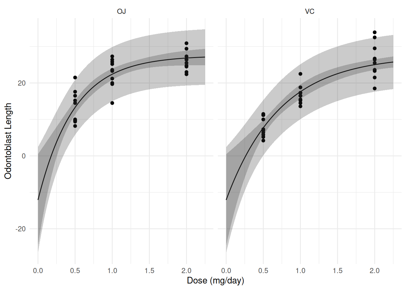
The nlsint function is also useful for plotting confidence and/or prediction intervals.

d <- expand.grid(supp = c("OJ", "VC"), dose = seq(0, 2.25, length = 100))
d <- cbind(d, nlsint(m, newdata = d))

p <- ggplot(ToothGrowth, aes(x = dose, y = len)) + 
  geom_point() + facet_wrap(~ supp) + theme_minimal() + 
  geom_line(aes(y = fit), data = d) + 
  geom_ribbon(aes(x = dose, ymin = lwr, ymax = upr, y = NULL), 
    alpha = 0.25, data = d) + 
  labs(x = "Dose (mg/day)", y = "Odontoblast Length")
plot(p)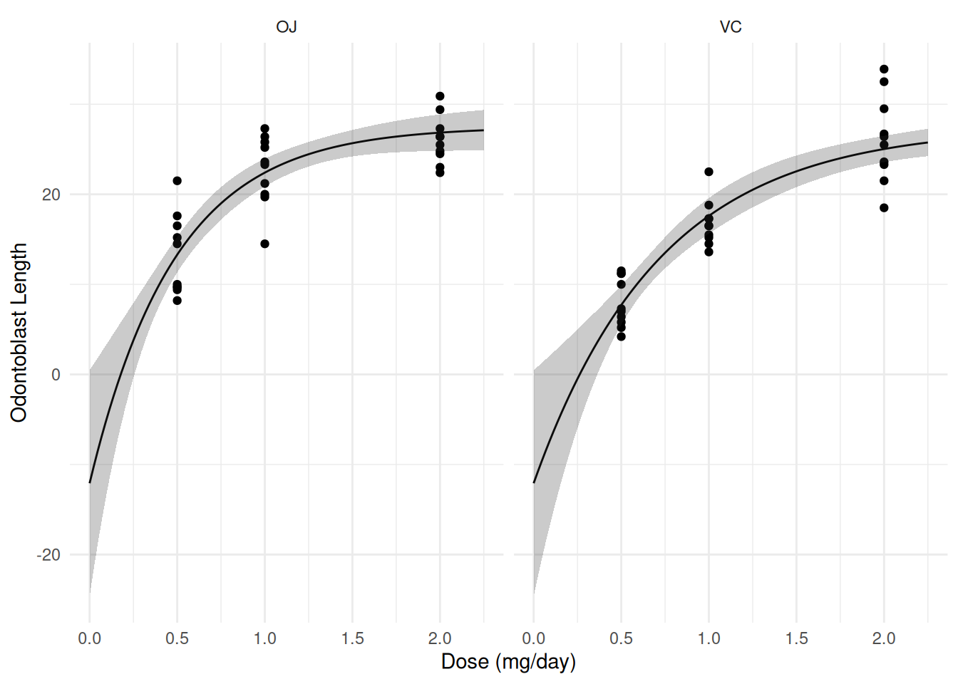

d <- expand.grid(supp = c("OJ", "VC"), dose = seq(0, 2.25, length = 100))
d <- cbind(d, nlsint(m, newdata = d, interval = "prediction"))
p <- p + geom_ribbon(aes(x = dose, ymin = lwr, ymax = upr, y = NULL), 
  alpha = 0.25, data = d)
plot(p)