Monday, February 3
You can also download a PDF copy of this lecture.
Modeling Nonlinearity
Four approaches to modeling a nonlinear relationship between the expected response and a quantitative explanatory variable.
polynomials
transformations
splines
nonlinear regression
The first three can be done with linear models.
Polynomial Regression
If we have a single explanatory variable \(x_i\), then a polynomial regression model of degree \(k\) is \[ E(Y_i) = \beta_0 + \beta_1 x_i + \beta_2 x_i^2 + \cdots + \beta_k x_i^k. \] Note that this is a linear model since we can write it as \[ E(Y_i) = \beta_0 + \beta_1 x_{i1} + \beta_2 x_{i2} + \cdots + \beta_k x_{ik}, \] where \(x_{i1} = x_i, x_{i2} = x_i^2, \dots, x_{ik} = x_i^k\).
Example: Consider again the ToothGrowth
data but with dose treated as a quantitative explanatory variable, and
ignoring supplement type for now. Note the use of the “inhibit” function
I here.
m <- lm(len ~ dose + I(dose^2), data = ToothGrowth)
summary(m)$coefficients
Estimate Std. Error t value Pr(>|t|)
(Intercept) -2.49 3.178 -0.7836 4.365e-01
dose 30.16 6.147 4.9052 8.148e-06
I(dose^2) -7.93 2.366 -3.3514 1.432e-03This model is \[ E(L_i) = \beta_0 + \beta_1 d_i + \beta_2 d_i^2, \] where \(d_i\) is dose.
d <- expand.grid(dose = seq(0.25, 2.25, length = 100))
d$yhat <- predict(m, newdata = d)

p <- ggplot(ToothGrowth, aes(x = dose, y = len)) +
  geom_point(aes(color = supp), alpha = 0.5) +
  geom_line(aes(y = yhat), data = d) +
  labs(x = "Dose (mg/day)", y = "Odontoblast Length",
    color = "Supplement Type") +
  theme_minimal() +
  theme(legend.position = "inside", legend.position.inside = c(0.8,0.2))
plot(p)
Note that the following are equivalent ways to specify this model.
# create a new variable for squared dose
ToothGrowth$dose2 <- ToothGrowth$dose^2
m <- lm(len ~ dose + dose2, data = ToothGrowth)

# specify squared dose in the model formula using the "inhibit" function
m <- lm(len ~ dose + I(dose^2), data = ToothGrowth)

# use the poly function to create the extra term
m <- lm(len ~ poly(dose, degree = 2), data = ToothGrowth)
I recommend not using the first approach of creating a new variable
only because it is easier to have the transformation “built in” to the
model when applying other functions to the model object like
predict or contrast.
Note: Using poly without the option
raw = TRUE will produce “orthogonal polynomials” which is a
re-parameterization of the model. This approach is sometimes recommended
due to numerical instability of “raw” polynomials, but in many cases
this is not an issue. But the poly function is sometimes
convenient, especially for polynomials of higher degree.
Clearly in such a model the rate of change in expected length is not necessarily constant.
library(trtools)
contrast(m, a = list(dose = 1), b = list(dose = 0.5)) # 0.5 to 1
estimate se lower upper tvalue df pvalue
9.13 1.341 6.444 11.82 6.806 57 6.697e-09contrast(m, a = list(dose = 1.5), b = list(dose = 1)) # 1 to 1.5 estimate se lower upper tvalue df pvalue
5.165 0.4472 4.27 6.06 11.55 57 1.47e-16This can also be seen mathematically by writing the model as \[ E(L_i) = \beta_0 + \beta_1x_i + \beta_2x_i^2 = \beta_0 + \underbrace{(\beta_1 + \beta_2x_i)}_{\delta_i}x_i = \beta_0 + \delta_ix_i, \] so that the rate of change in length per unit increase in dose depends on dose (if \(\beta_2 \neq 0\)). In a sense, dose is “interacting with itself” — i.e., the “effect” of a one unit increase in dose depends on the dose.
We can have the polynomial depend on (i.e, interact with) supplement type.
m <- lm(len ~ dose + I(dose^2) + supp + dose:supp + I(dose^2):supp, data = ToothGrowth)
summary(m)$coefficients
Estimate Std. Error t value Pr(>|t|)
(Intercept) -1.433 3.847 -0.3726 7.109e-01
dose 34.520 7.442 4.6384 2.272e-05
I(dose^2) -10.387 2.864 -3.6260 6.383e-04
suppVC -2.113 5.440 -0.3885 6.992e-01
dose:suppVC -8.730 10.525 -0.8295 4.105e-01
I(dose^2):suppVC 4.913 4.051 1.2129 2.305e-01Note that we could also have written
m <- lm(len ~ poly(dose, 2)*supp, data = ToothGrowth)In a model formula argument, a*b expands to
a + b + a:b.
This model can be written as \[ E(L_i) = \begin{cases} \beta_0 + \beta_1 d_i + \beta_2 d_i^2, & \text{if supplement type is OJ}, \\ \beta_0 + \beta_3 + (\beta_1 + \beta_4) d_i + (\beta_2 + \beta_5) d_i^2, & \text{if supplement type is VC}, \end{cases} \] where \(d_i\) is dose, or alternatively as \[ E(L_i) = \begin{cases} \beta_0 + \beta_1 d_i + \beta_2 d_i^2, & \text{if supplement type is OJ}, \\ \gamma_0 + \gamma_1 d_i + \gamma_2 d_i^2, & \text{if supplement type is VC}, \end{cases} \] where \(\gamma_0 = \beta_0 + \beta_3\), \(\gamma_1 = \beta_1 + \beta_4\), and \(\gamma_2 = \beta_2 + \beta_5\). There is a distinct polynomial of degree two for each supplement type.
d <- expand.grid(supp = c("OJ", "VC"), dose = seq(0.25, 2.25, length = 100))
d$yhat <- predict(m, newdata = d)
p <- ggplot(ToothGrowth, aes(x = dose, y = len, color = supp)) +
geom_point(alpha = 0.5) + geom_line(aes(y = yhat), data = d) +
labs(x = "Dose (mg/day)", y = "Odontoblast Length",
color = "Supplement Type") + theme_minimal() +
theme(legend.position = "inside", legend.position.inside = c(0.8,0.2))
plot(p)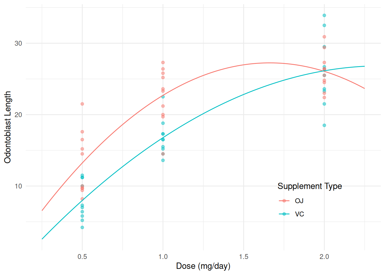 Polynomials are, in principle, quite general. But in many cases we would
like to have a monotonic relationship, and/or have a model exhibit an
asymptote. Finally, the parameters of a polynomial model are not easily
to interpret.
Polynomials are, in principle, quite general. But in many cases we would
like to have a monotonic relationship, and/or have a model exhibit an
asymptote. Finally, the parameters of a polynomial model are not easily
to interpret.
Logarithmic Transformations
Applying a logarithmic transformation to an explanatory variable may be useful for explanatory variables that tend to have “diminishing returns” with respect to the expected response.
Example: Consider a linear model for expected length but now with \(\log(\text{dose})\) as the explanatory variable.
m <- lm(len ~ log(dose) + supp + log(dose):supp, data = ToothGrowth)
summary(m)$coefficients
Estimate Std. Error t value Pr(>|t|)
(Intercept) 20.663 0.6791 30.425 1.629e-36
log(dose) 9.255 1.2000 7.712 2.303e-10
suppVC -3.700 0.9605 -3.852 3.033e-04
log(dose):suppVC 3.845 1.6971 2.266 2.737e-02d <- expand.grid(supp = c("OJ", "VC"), dose = seq(0.25, 2.25, length = 100))
d$yhat <- predict(m, newdata = d)
p <- ggplot(ToothGrowth, aes(x = dose, y = len, color = supp)) +
geom_point(alpha = 0.5) + geom_line(aes(y = yhat), data = d) +
labs(x = "Dose (mg/day)", y = "Odontoblast Length",
color = "Supplement Type") + theme_minimal() +
theme(legend.position = "inside", legend.position.inside = c(0.8,0.2))
plot(p) Note that
 log is the “natural” logarithm or base-\(e\) logarithm sometimes written as \(\ln(x)\) or \(\log_e(x)\). Here are few things to
remember about logarithms when using them for transformations of
explanatory variables.
Logarithms of different bases are proportional. In general \[ \log_b(x) = c\log_a(x), \] where \(c = 1/\log_a(b)\). So usually when we are using things like
contrastor the emmeans package to facilitate our inferences the base does not matter. You can uselog2for \(\log_2(x)\) andlog10for \(\log_{10}(x)\), and for an arbitrary base \(b\) you can uselog(x,b)for \(\log_b(x)\).m <- lm(len ~ log2(dose) + supp + log2(dose):supp, data = ToothGrowth) summary(m)$coefficientsEstimate Std. Error t value Pr(>|t|) (Intercept) 20.663 0.6791 30.425 1.629e-36 log2(dose) 6.415 0.8318 7.712 2.303e-10 suppVC -3.700 0.9605 -3.852 3.033e-04 log2(dose):suppVC 2.665 1.1763 2.266 2.737e-02d <- expand.grid(supp = c("OJ", "VC"), dose = seq(0.25, 2.25, length = 100)) d$yhat <- predict(m, newdata = d) p <- ggplot(ToothGrowth, aes(x = dose, y = len, color = supp)) + geom_point(alpha = 0.5) + geom_line(aes(y = yhat), data = d) + labs(x = "Dose (mg/day)", y = "Odontoblast Length", color = "Supplement Type") + theme_minimal() + theme(legend.position = "inside", legend.position.inside = c(0.8,0.2)) plot(p)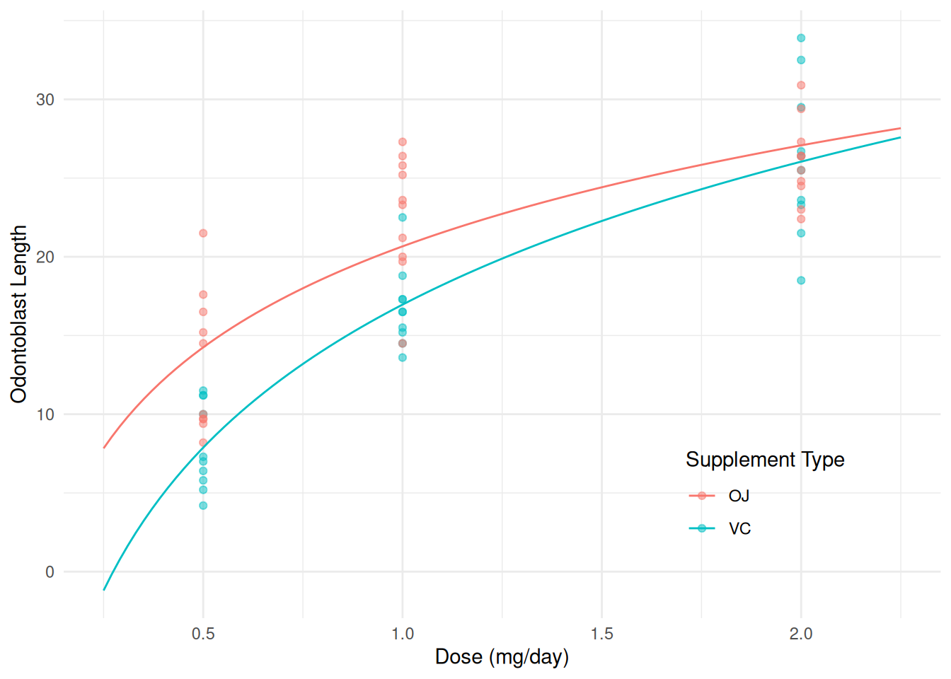
If we apply a log transformation to \(x\), then the effect of increasing/decreasing \(x\) by some amount is not constant, but the effect of increasing/decreasing \(x\) by a factor is constant. For example, suppose we have the model \[ E(Y) = \beta_0 + \beta_1 \log(x). \]
Then for any \(c > 0\) then \[ \beta_0 + \beta_1\log(cx) = \beta_0 + \beta_1\log(c) + \beta_1\log(x) = E(Y) + \beta_1\log(c) \] so then \(E(Y)\) increases/decreases by \(\beta_1\log(c)\). For example, the effect of doubling of halving dose is constant in this model.contrast(m, a = list(dose = 1, supp = c("OJ","VC")), b = list(dose = 0.5, supp = c("OJ","VC")), cnames = c("OJ", "VC"))estimate se lower upper tvalue df pvalue OJ 6.415 0.8318 4.749 8.081 7.712 56 2.303e-10 VC 9.080 0.8318 7.414 10.746 10.916 56 1.733e-15contrast(m, a = list(dose = 2, supp = c("OJ","VC")), b = list(dose = 1, supp = c("OJ","VC")), cnames = c("OJ", "VC"))estimate se lower upper tvalue df pvalue OJ 6.415 0.8318 4.749 8.081 7.712 56 2.303e-10 VC 9.080 0.8318 7.414 10.746 10.916 56 1.733e-15Recall that \(\log(x)\) is only defined for \(x > 0\).
Exponential Transformations
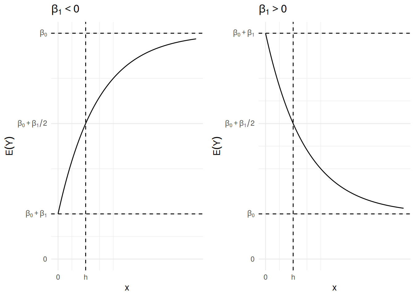
Consider the linear model \[ E(Y) = \beta_0 + \beta_12^{-x/h} \] where \(h > 0\) is some specified value. This applies an exponential transformation to \(x\) with the following properties.
If \(x = 0\) then \(E(Y) = \beta_0 + \beta_1\), so the “\(y\)-intercept” is \(\beta_0 + \beta_1\).
As \(x\) increases then \(E(Y)\) approaches an asymptote of \(\beta_0\). This is an upper (if \(\beta_1 < 0\)) or lower (if \(\beta_1 > 0\)) asymptote.1
The quantity \(h\) can be interpreted as the “half-life” of the curve in the sense that it is the value of \(x\) at which the expected responses is half way between the intercept at \(\beta_0 + \beta_1\) and its upper/lower asymptote at \(\beta_0\) because if \(x = h\) then \[ E(Y) = \beta_0 + \beta_12^{-x/h} = \beta_0 + \beta_1/2, \] and \(\beta_0 + \beta_1/2\) is the midpoint between the “intercept” of \(E(Y) = \beta_0 + \beta_1\) and the asymptote of \(\beta_0\).
If \(\beta_1 < 0\) then \(-\beta_1\) is how much \(E(Y)\) increases from \(x = 0\) as it approaches the asymptote, while if \(\beta_1 > 0\) then \(\beta_1\) is how much \(E(Y)\) decreases from when \(x = 0\) as it approaches the asymptote.
Consider again a linear model for the ToothGrowth data
with an exponential transformation of dose with \(h\) = 1.
m <- lm(len ~ I(2^(-dose/1)), data = ToothGrowth)
summary(m)$coefficients
Estimate Std. Error t value Pr(>|t|)
(Intercept) 35.14 1.555 22.60 1.942e-30
I(2^(-dose/1)) -33.61 2.988 -11.25 3.303e-16d <- expand.grid(supp = c("OJ", "VC"), dose = seq(0, 6, length = 100))
d$yhat <- predict(m, newdata = d)
p <- ggplot(ToothGrowth, aes(x = dose, y = len, color = supp)) +
geom_point(alpha = 0.5) + xlim(0,6) +
geom_line(aes(y = yhat), color = "black", data = d) +
labs(x = "Dose (mg/day)", y = "Odontoblast Length",
color = "Supplement Type") + theme_minimal() +
theme(legend.position = "inside", legend.position.inside = c(0.8,0.2))
plot(p)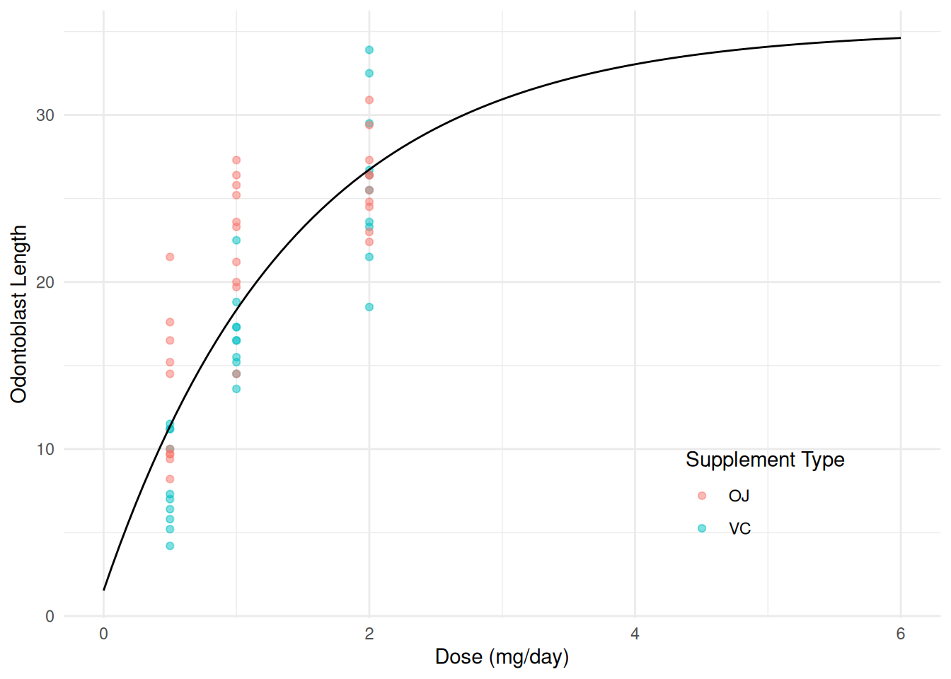
lincon(m, a = c(1,1)) # intercept estimate se lower upper tvalue df pvalue
(1,1),0 1.528 1.635 -1.745 4.8 0.9345 58 0.3539Now suppose that we let the effect of dose “interact” with supplement type.
m <- lm(len ~ I(2^(-dose/1)) + supp + supp:I(2^(-dose/1)), data = ToothGrowth)
summary(m)$coefficients
Estimate Std. Error t value Pr(>|t|)
(Intercept) 34.054 1.925 17.6872 1.375e-24
I(2^(-dose/1)) -27.569 3.700 -7.4519 6.199e-10
suppVC 2.169 2.723 0.7964 4.291e-01
I(2^(-dose/1)):suppVC -12.083 5.232 -2.3094 2.463e-02d <- expand.grid(supp = c("OJ", "VC"), dose = seq(0, 6, length = 100))
d$yhat <- predict(m, newdata = d)
p <- ggplot(ToothGrowth, aes(x = dose, y = len, color = supp)) +
geom_point(alpha = 0.5) + xlim(0,6) +
geom_line(aes(y = yhat), data = d) +
labs(x = "Dose (mg/day)", y = "Odontoblast Length",
color = "Supplement Type") + theme_minimal() +
theme(legend.position = "inside", legend.position.inside = c(0.8,0.2))
plot(p)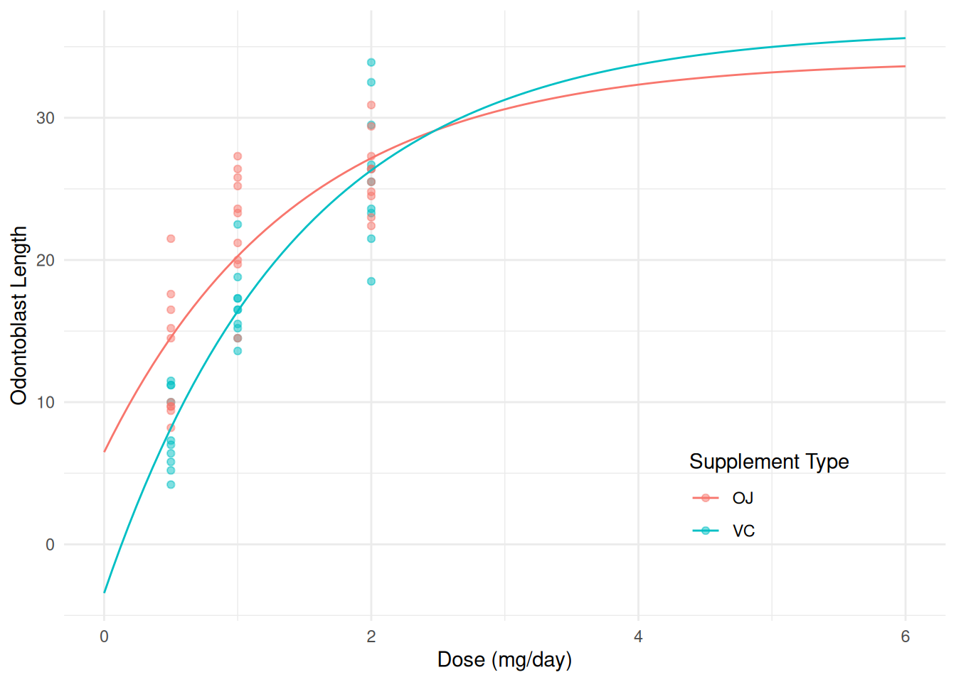 This model can be written as \[
E(Y_i) = \beta_0 + \beta_12^{-x_i/h} + \beta_2d_i +
\beta_3d_i2^{-x_i/h},
\] where \(d_i\) = 1 if the
supplement type is VC, and \(d_i\) = 0
otherwise, and \(h\) = 1. We can also
write this model case-wise as \[
E(Y_i) =
\begin{cases}
\beta_0 + \beta_12^{-x_i/h}, & \text{if the supplement type
of the $i$-th observation is OJ}, \\
\beta_0 + \beta_2 + (\beta_1 + \beta_3)2^{-x_i/h}, &
\text{if the supplement type of the $i$-th observation is VC},
\end{cases}
\] or \[
E(Y_i) =
\begin{cases}
\beta_0 + \beta_12^{-x_i/h}, & \text{if the supplement type
of the $i$-th observation is OJ}, \\
\gamma_0 + \gamma_12^{-x_i/h}, & \text{if the supplement
type of the $i$-th observation is VC},
\end{cases}
\] where \(\gamma_0 = \beta_0 +
\beta_2\) and \(\gamma_1 = \beta_1 +
\beta_3\). We can make inferences for the intercepts and
asymptotes for each supplement type using
This model can be written as \[
E(Y_i) = \beta_0 + \beta_12^{-x_i/h} + \beta_2d_i +
\beta_3d_i2^{-x_i/h},
\] where \(d_i\) = 1 if the
supplement type is VC, and \(d_i\) = 0
otherwise, and \(h\) = 1. We can also
write this model case-wise as \[
E(Y_i) =
\begin{cases}
\beta_0 + \beta_12^{-x_i/h}, & \text{if the supplement type
of the $i$-th observation is OJ}, \\
\beta_0 + \beta_2 + (\beta_1 + \beta_3)2^{-x_i/h}, &
\text{if the supplement type of the $i$-th observation is VC},
\end{cases}
\] or \[
E(Y_i) =
\begin{cases}
\beta_0 + \beta_12^{-x_i/h}, & \text{if the supplement type
of the $i$-th observation is OJ}, \\
\gamma_0 + \gamma_12^{-x_i/h}, & \text{if the supplement
type of the $i$-th observation is VC},
\end{cases}
\] where \(\gamma_0 = \beta_0 +
\beta_2\) and \(\gamma_1 = \beta_1 +
\beta_3\). We can make inferences for the intercepts and
asymptotes for each supplement type using
lincon.
lincon(m, a = c(1,1,0,0)) # b0 + b1 = intercept for OJ estimate se lower upper tvalue df pvalue
(1,1,0,0),0 6.485 2.024 2.429 10.54 3.203 56 0.002243lincon(m, a = c(1,1,1,1)) # g0 + g1 = b0 + b2 + b1 + b3 = intercept for VC estimate se lower upper tvalue df pvalue
(1,1,1,1),0 -3.429 2.024 -7.485 0.6261 -1.694 56 0.09582lincon(m, a = c(1,0,1,0)) # g0 = b0 + b2 = asymptote for VC estimate se lower upper tvalue df pvalue
(1,0,1,0),0 36.22 1.925 32.37 40.08 18.81 56 7.07e-26We can also obtain (approximate) inferences using
contrast.
contrast(m, a = list(dose = 0, supp = c("OJ","VC")),
    cname = c("OJ intercept","VC intercept"))
estimate se lower upper tvalue df pvalue
OJ intercept 6.485 2.024 2.429 10.5401 3.203 56 0.002243
VC intercept -3.429 2.024 -7.485 0.6261 -1.694 56 0.095824contrast(m, a = list(dose = 100, supp = c("OJ","VC")),
cname = c("OJ asymptote","VC asymptote")) estimate se lower upper tvalue df pvalue
OJ asymptote 34.05 1.925 30.20 37.91 17.69 56 1.375e-24
VC asymptote 36.22 1.925 32.37 40.08 18.81 56 7.070e-26But wouldn’t it make sense to have something like the following? \[ E(Y_i) = \begin{cases} \beta_0 + \beta_12^{-x_i/h_{\text{OJ}}}, & \text{if the supplement type of the $i$-th observation is OJ}, \\ \beta_0 + \beta_12^{-x_i/h_{\text{VC}}}, & \text{if the supplement type of the $i$-th observation is VC}, \end{cases} \] because at \(x = 0\) and as \(x \rightarrow \infty\) there should be no difference in the supplement type, but there might be a difference in how “fast” the expected response increases with dose. But unless we know \(h_{\text{OJ}}\) and \(h_{\text{VC}}\), this model would be nonlinear (i.e., the model is not linear if \(h_{\text{OJ}}\) and \(h_{\text{VC}}\) are unknown parameters as opposed to known values).
This can be seen by showing that \(\lim_{x \to \infty} \beta_0 + \beta_12^{-x/h} = \beta_0\) if \(h > 0\), and by showing that the first derivative of \(\beta_0 + \beta_12^{-x/h}\) with respect to \(x\) is positive if \(\beta_1 < 0\) and negative if \(\beta_1 > 0\) if \(h > 0\).↩︎