Wednesday, April 30
You can also download a PDF copy of this lecture.
Generalized Additive Models
Consider models of the form \[ g[E(Y)] = \beta_0 + f(x) \] or \[ g[E(Y)] = \beta_0 + f_1(x_1) + f_2(x_2) \] or \[ g[E(Y)] = \beta_0 + f(x_1,x_2) \] or \[ g[E(Y)] = \beta_0 + f_1(x_1) + f_2(x_2,x_3), \] where \(g\) is a link function and \(f\), \(f_1\), and \(f_2\) are functions. Linear and generalized linear models are special cases of GAMs. But the term GAM usually refers to cases where the functions of the explanatory variables are specified to be flexible but smooth functions. Splines are frequently used for these functions.
Splines
A spline can be viewed a couple of different ways.
A function made up of several polynomial functions that join at a set of knots.
Example: A cubic spline for a linear model with knots \(\zeta_1\) and \(\zeta_2\) can be written as \[ E(Y) = \begin{cases} \delta_0 + \delta_1 x + \delta_2 x^2 + \delta_3 x^3, & \text{if $x < \zeta_1$}, \\ \delta_0 + \delta_1 x + \delta_2 x^2 + \delta_3 x^3 + \delta_4(x-\zeta_1)^3, & \text{if $\zeta_1 \le x < \zeta_2$} \\ \delta_0 + \delta_1 x + \delta_2 x^2 + \delta_3 x^3 + \delta_4(x-\zeta_1)^3 + \delta_5(x-\zeta_2)^3, & \text{if $\zeta_2 \le x$}. \end{cases} \] Here is cubic spline as a regression model.
library(MASS) # for the mcycle data
library(splines) # for the bs function
m <- lm(accel ~ bs(times, knots = c(20,40)), data = mcycle)
summary(m)$coefficients
Estimate Std. Error t value Pr(>|t|) (Intercept) -15.2 16.4 -0.93 3.54e-01 bs(times, knots = c(20, 40))1 86.0 28.4 3.03 2.95e-03 bs(times, knots = c(20, 40))2 -201.3 20.7 -9.71 5.26e-17 bs(times, knots = c(20, 40))3 199.0 29.5 6.74 4.97e-10 bs(times, knots = c(20, 40))4 -110.1 27.8 -3.96 1.23e-04 bs(times, knots = c(20, 40))5 67.6 29.6 2.29 2.38e-02d <- data.frame(times = seq(2.4, 57.6, length = 1000)) d$yhat <- predict(m, newdata = d) p <- ggplot(mcycle, aes(x = times, y = accel)) + geom_point() + theme_classic() + labs(x = "Time After Impact (ms)", y = "Head Acceleration (g)") + geom_vline(xintercept = c(20,40), linetype = 3) + geom_line(aes(y = yhat), data = d) plot(p)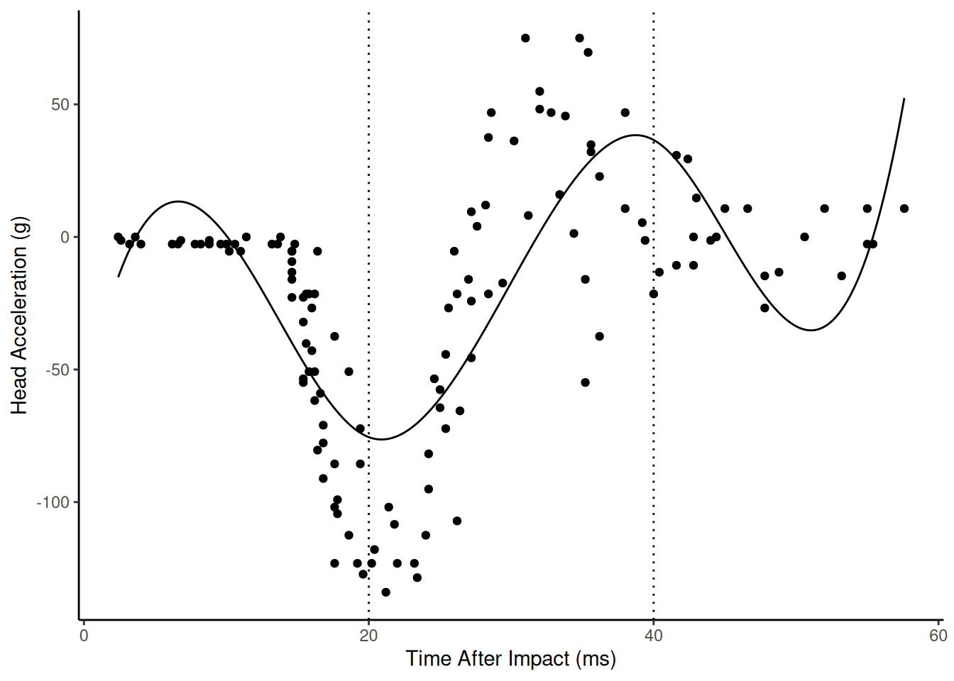
A function that is a weighted average of a set of basis functions such that \[ f(x) = \sum_j \delta_j b_j(x), \] where \(b_j(x)\) is the \(j\)-th basis function and \(\delta_j\) is a parameter. The spline shown above can be written in terms of five basis functions.
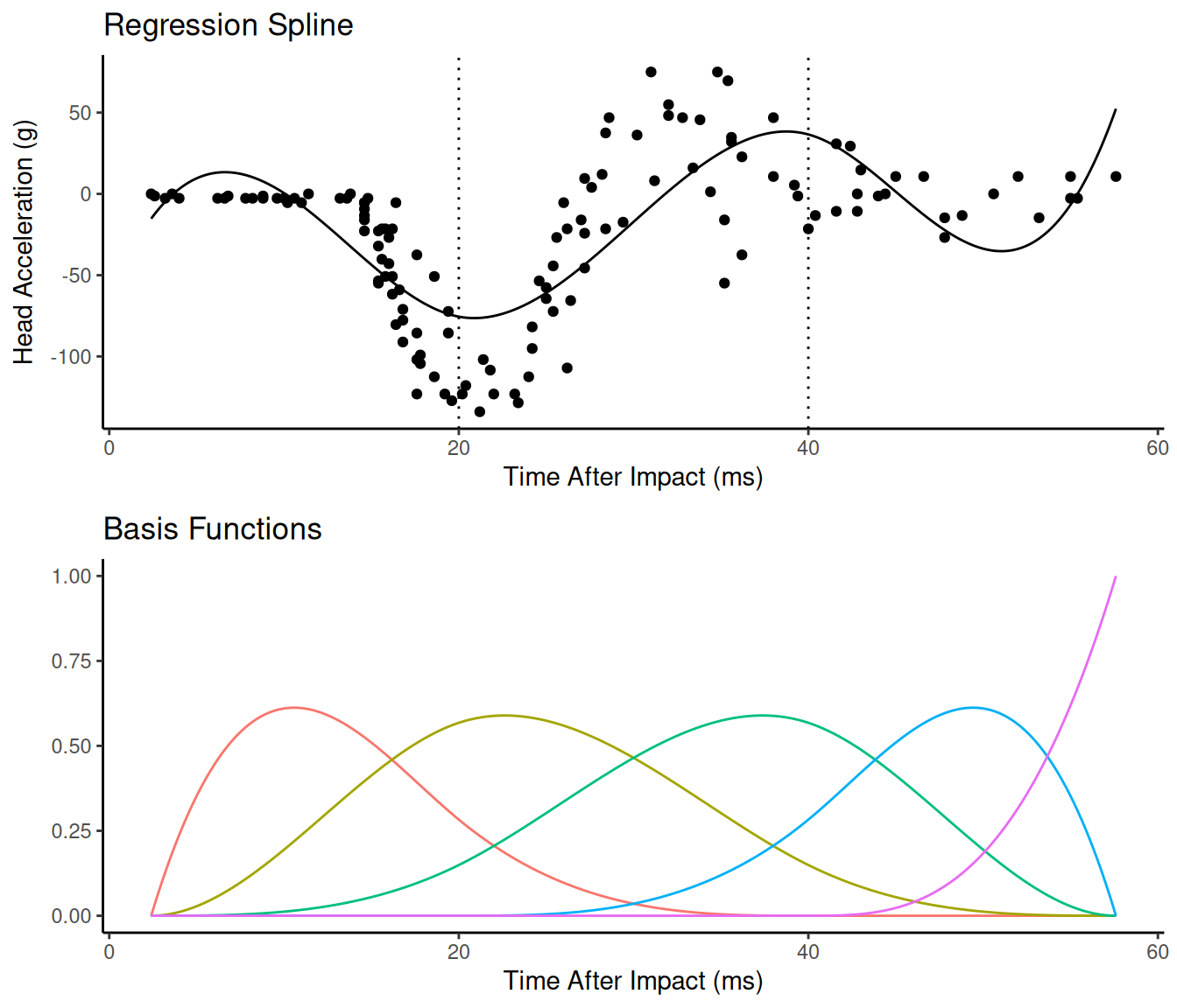 So the model can be written as \[
E(Y) = \beta_0 + \sum_{j=1}^5\delta_jb_j(x) = \beta_0 + \beta_1 x_1^*
+ \beta_2 x_2^* + \beta_3 x_3^* + \beta_4 x_4^* + \beta_5 x_5^*,
\] where \(\delta_j = \beta_j\)
and \(x_j^* = b_j(x)\). Because this is
still a (generalized) linear model, it is still quite tractable
computationally and theoretically (provided we treat the number and
placement of knots as well as the form of the functions as
known).
So the model can be written as \[
E(Y) = \beta_0 + \sum_{j=1}^5\delta_jb_j(x) = \beta_0 + \beta_1 x_1^*
+ \beta_2 x_2^* + \beta_3 x_3^* + \beta_4 x_4^* + \beta_5 x_5^*,
\] where \(\delta_j = \beta_j\)
and \(x_j^* = b_j(x)\). Because this is
still a (generalized) linear model, it is still quite tractable
computationally and theoretically (provided we treat the number and
placement of knots as well as the form of the functions as
known).
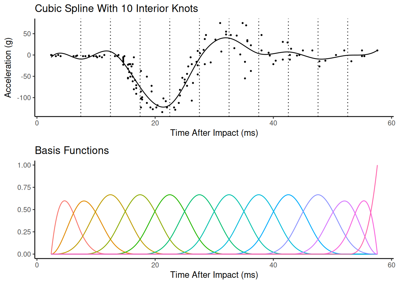
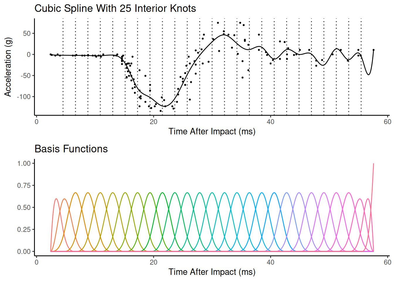
Spline Complexity
The spline can be made more flexible by adding more knots or basis functions. Adding more knots or basis functions makes the spline more flexible, but potentially too flexible. This is a bias-variance trade-off.

 In principle we could use cross-validation or a related technique
(e.g. AIC) to try to identify a good trade-off. But a better approach is
to use penalization/regularization.
In principle we could use cross-validation or a related technique
(e.g. AIC) to try to identify a good trade-off. But a better approach is
to use penalization/regularization.
Penalized Splines
Instead of trying to select the number of knots or basis functions, we could specify a “generous” number of knots/functions and introduce a penalty for “wiggliness” in the estimation. Suppose we have the model \[ E(Y_i) = \beta_0 + f(x_i), \] where \(f\) is a spline such that \[ f(x_i) = \sum_j \delta_j b_j(x_i). \] Then using (weighted) least squares we can try to minimize \[ \sum_{i=1}^n w_i(y_i - \hat{y}_i)^2 + \lambda h(f). \] where \(\lambda \ge 0\) and \(h\) is a function that measures the “wiggliness” of the function \(f\). One reasonable measure of “wiggliness” is to integrate over the second derivative of \(f\) such that \[ h(f) = \! \int f''(x)^2 dx. \] Fortunately this function can be written in a relatively simple way so that it is relatively easy to compute and solve the (penalized) least squares problem. The control over the flexibility/wiggliness of the spline is then through \(\lambda\). As \(\lambda\) increases \(f\) approaches a line, but as \(\lambda\) approaches zero then \(f\) becomes increasingly flexible/wiggly.
Example: Using the gam function from
the mgcv package allows us to control the wiggliness
through the sp argument. Here is “maximum wiggliness”.
library(mgcv) # for the gam and supporting functions
knots <- seq(2.4, 57.6, length = 27)
m <- gam(accel ~ s(times, bs = "bs", k = length(knots), sp = 0),
data = mcycle, knots = list(x = knots))
d <- data.frame(times = seq(2.4, 57.6, length = 1000))
d$yhat <- predict(m, newdata = d)
p <- ggplot(mcycle, aes(x = times, y = accel)) + theme_classic() +
geom_point() + labs(x = "Time After Impact (ms)", y = "Acceleration (g)") +
geom_line(aes(y = yhat), data = d) + geom_vline(xintercept = knots, linetype = 3)
plot(p)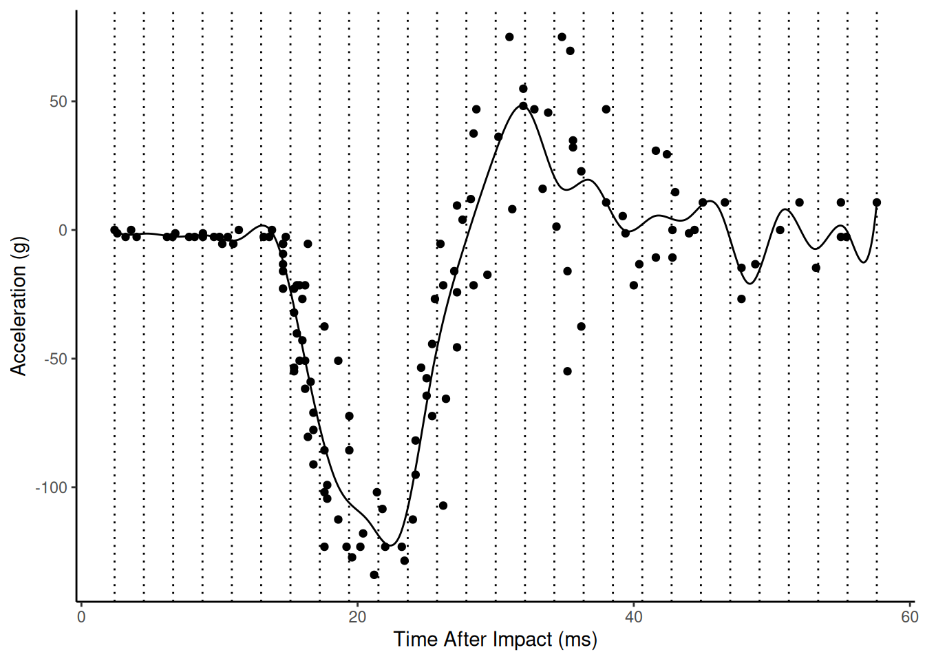 Here is the estimated model with
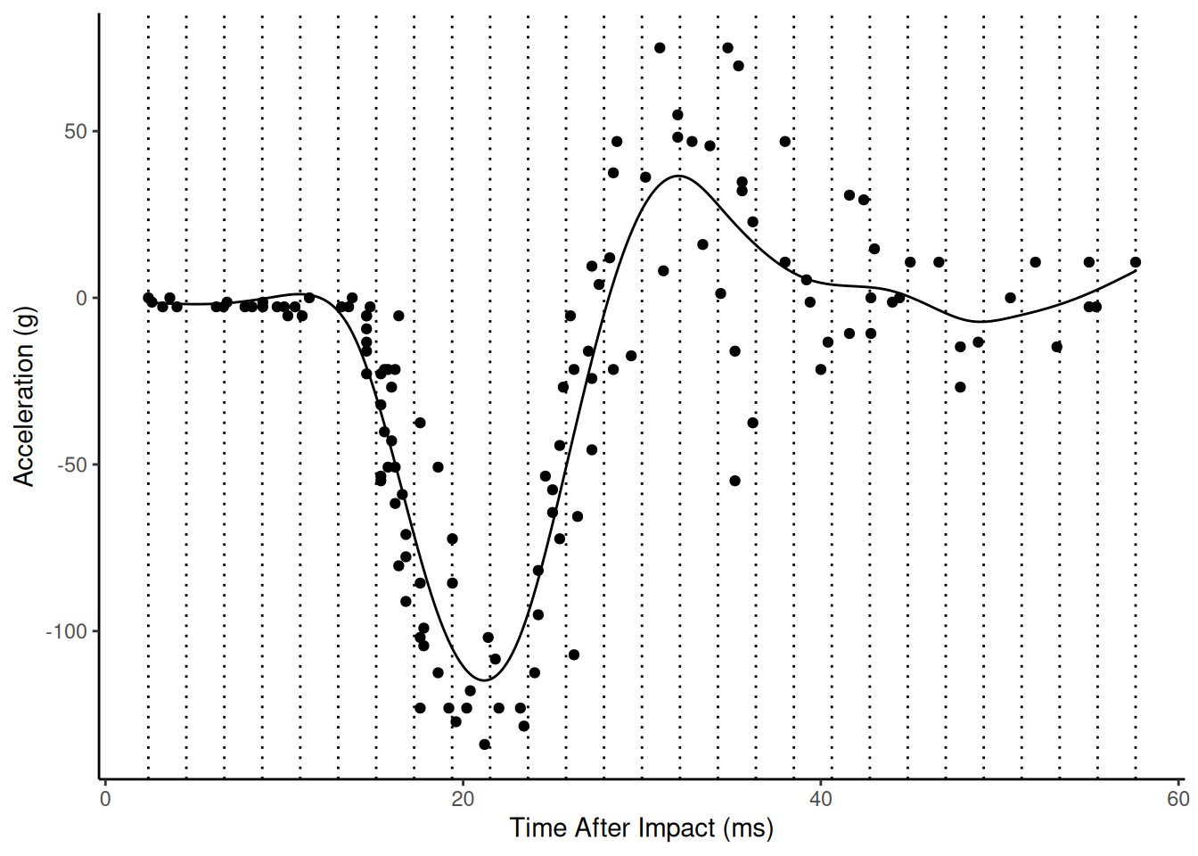
 sp = 10.
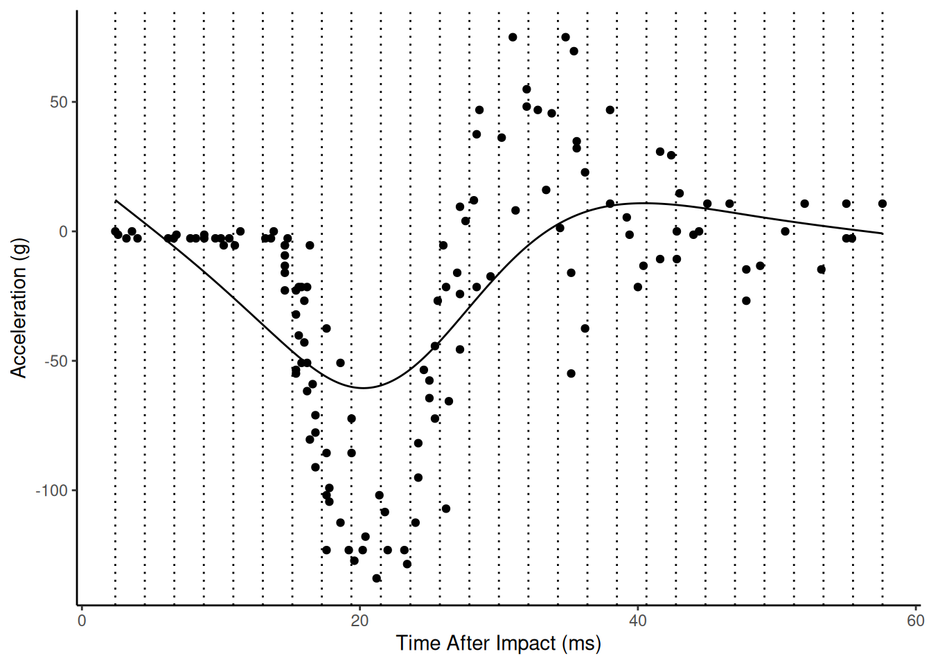
 Here is the estimated model with
 sp = 1000.
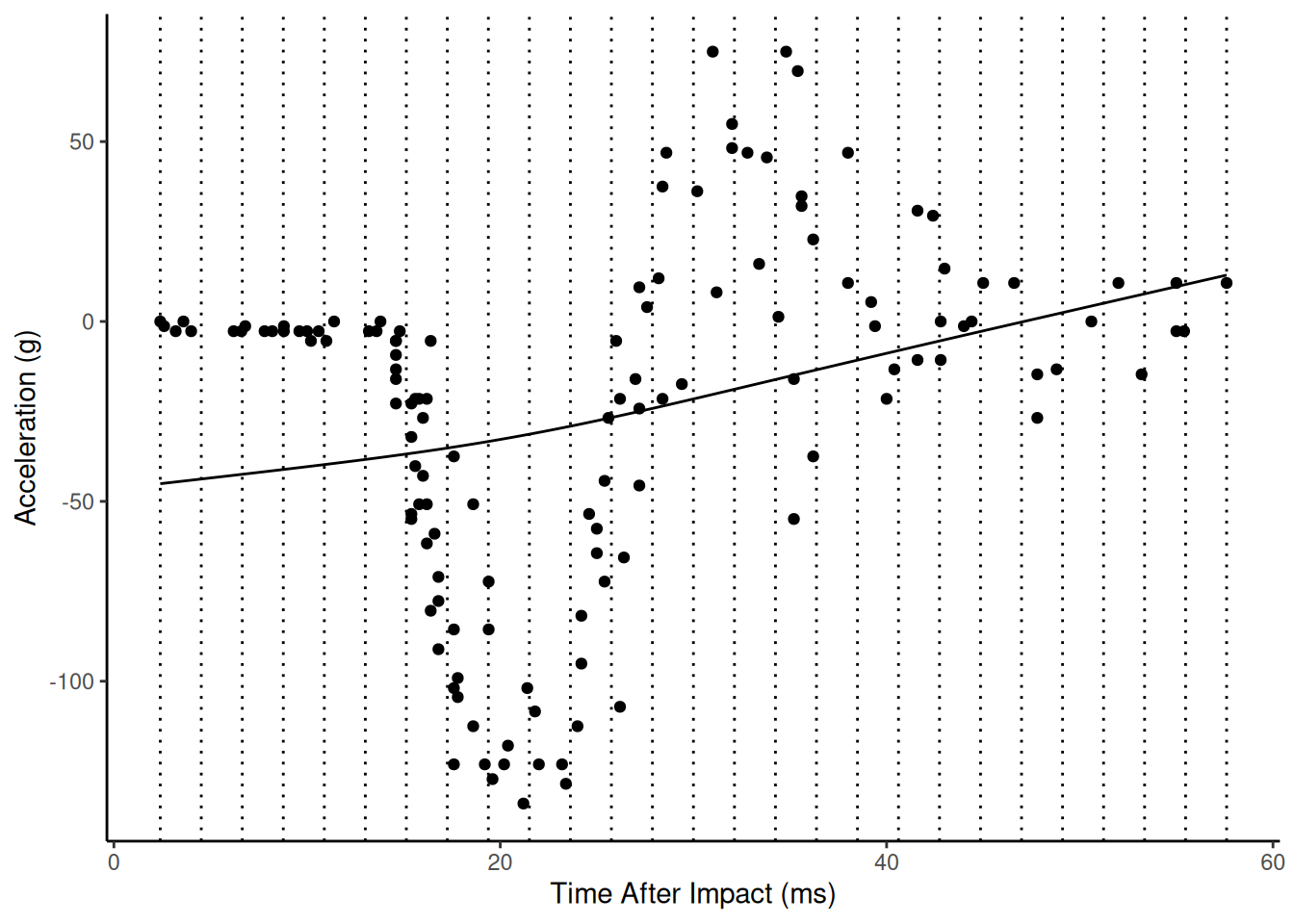
 Here is the estimated model with
 sp = 100000 (nearly
minimum wiggliness).
 The mgcv package gives the user access to a wide
variety of types of splines and ways to modify them. But it also
provides “automatic” cross-validation and selection of \(\lambda\) using a generalized
cross-validation (GCV) measure.
The mgcv package gives the user access to a wide
variety of types of splines and ways to modify them. But it also
provides “automatic” cross-validation and selection of \(\lambda\) using a generalized
cross-validation (GCV) measure.
Example: Consider again the mcycles
data. Here we will use the default settings.
m <- gam(accel ~ s(times), data = mcycle)
summary(m)
Family: gaussian
Link function: identity

Formula:
accel ~ s(times)

Parametric coefficients:
            Estimate Std. Error t value Pr(>|t|)
(Intercept)   -25.55       1.95   -13.1   <2e-16 ***
---
Signif. codes:  0 '***' 0.001 '**' 0.01 '*' 0.05 '.' 0.1 ' ' 1

Approximate significance of smooth terms:
          edf Ref.df    F p-value
s(times) 8.69   8.97 53.5  <2e-16 ***
---
Signif. codes:  0 '***' 0.001 '**' 0.01 '*' 0.05 '.' 0.1 ' ' 1

R-sq.(adj) =  0.783   Deviance explained = 79.8%
GCV = 545.78  Scale est. = 506       n = 133
d <- data.frame(times = seq(2.4, 57.6, length = 1000))
d$yhat <- predict(m, newdata = d)
p <- ggplot(mcycle, aes(x = times, y = accel)) + theme_classic() +
geom_point() + labs(x = "Time After Impact (ms)", y = "Acceleration (g)") +
geom_line(aes(y = yhat), data = d) +
geom_vline(xintercept = knots, linetype = 3)
plot(p)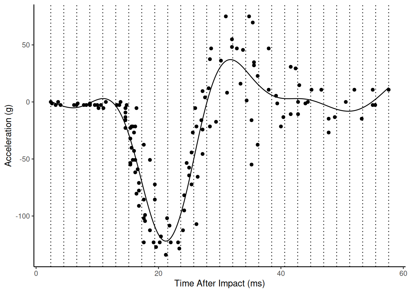
Example: Consider the bone data that
shows relative bone mineral density by age and sex.
bone <- read.table("http://faculty.washington.edu/jonno/book/spinalbonedata.txt", header = TRUE)
m <- gam(spnbmd ~ s(age), data = bone)

d <- expand.grid(sex = c("fem","mal"), age = seq(9, 26, length = 1000))
d$yhat <- predict(m, newdata = d)

p <- ggplot(bone, aes(x = age, y = spnbmd)) +
  geom_point(aes(color = sex), alpha = 0.25) + theme_classic() +
  geom_line(aes(color = sex, group = idnum), alpha = 0.25) +
  labs(x = "Age (years)", color = "Sex",
    y = "Relative Spinal Bone Mineral Density") +
  geom_line(aes(y = yhat), data = d)
plot(p)
m <- gam(spnbmd ~ sex + s(age), data = bone)

d <- expand.grid(sex = c("fem","mal"), age = seq(9, 26, length = 1000))
d$yhat <- predict(m, newdata = d)

p <- ggplot(bone, aes(x = age, y = spnbmd)) +
  geom_point(aes(color = sex), alpha = 0.25) + theme_classic() +
  geom_line(aes(color = sex, group = idnum), alpha = 0.25) +
  labs(x = "Age (years)", color = "Sex",
    y = "Relative Spinal Bone Mineral Density") +
  geom_line(aes(y = yhat, color = sex), data = d)
plot(p)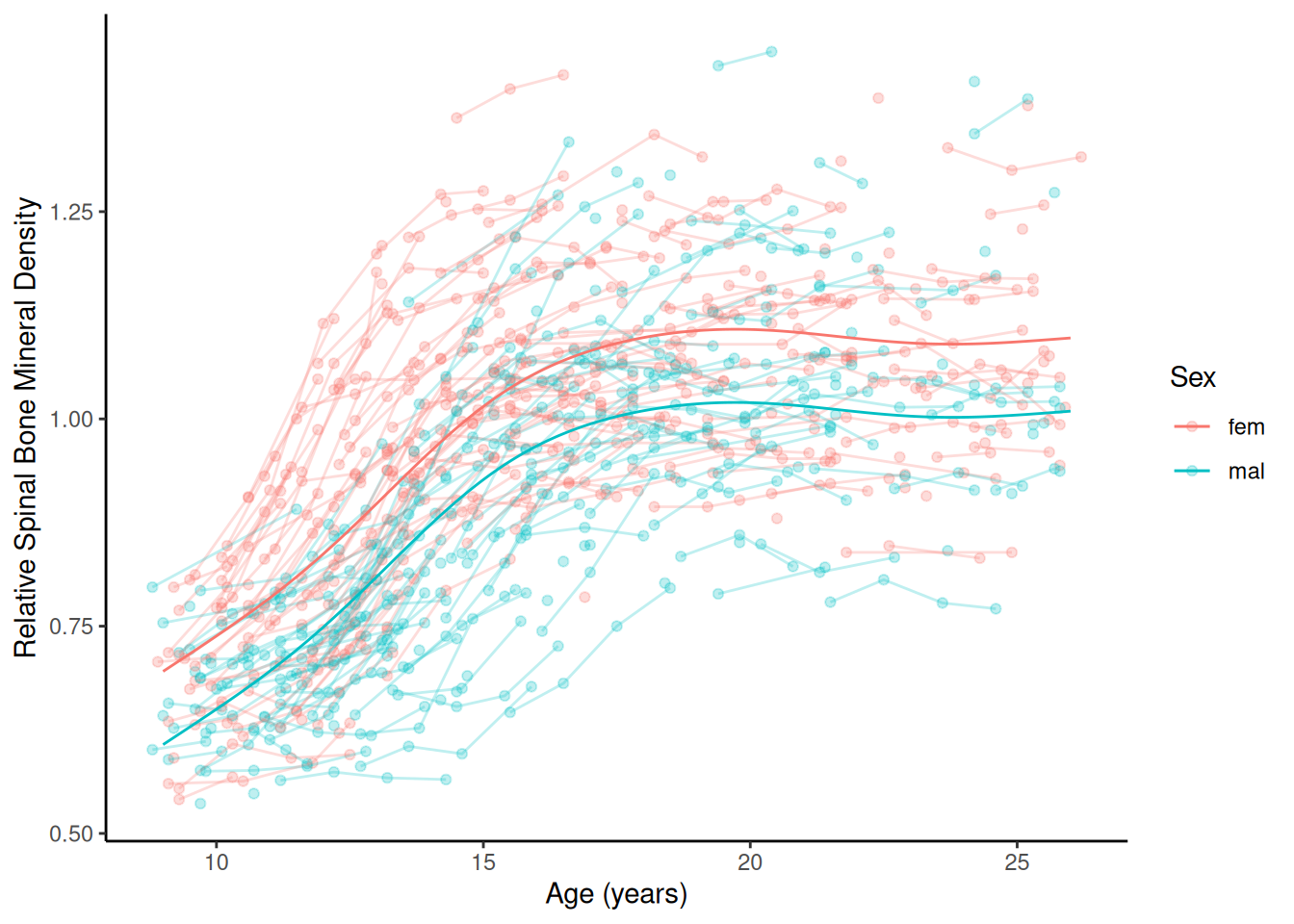
m <- gam(spnbmd ~ sex + s(age, by = factor(sex)), data = bone)

d <- expand.grid(sex = c("fem","mal"), age = seq(9, 26, length = 1000))
d$yhat <- predict(m, newdata = d)

p <- ggplot(bone, aes(x = age, y = spnbmd)) +
  geom_point(aes(color = sex), alpha = 0.25) + theme_classic() +
  geom_line(aes(color = sex, group = idnum), linewidth = 0.5, alpha = 0.25) +
  labs(x = "Age (years)", color = "Sex",
    y = "Relative Spinal Bone Mineral Density") +
  geom_line(aes(y = yhat, color = sex), data = d)
plot(p) Example: Consider the growth data of female and male
children in the
Example: Consider the growth data of female and male
children in the children data frame from the
npregfast package. Here I am adding a confidence band
to each function.
library(npregfast)
m <- gam(height ~ sex + s(age, by = factor(sex)), data = children)

d <- expand.grid(age = seq(5, 19, length = 1000),
  sex = c("female","male"))
d$yhat <- predict(m, newdata = d)
d$se <- predict(m, newdata = d, se.fit = TRUE)$se.fit
d$lower <- d$yhat - 2*d$se
d$upper <- d$yhat + 2*d$se

p <- ggplot(children, aes(x = age, y = height)) + theme_classic() +
  geom_point(aes(color = sex), size = 0.25, alpha = 0.25) +
  geom_line(aes(y = yhat, color = sex), data = d) +
  geom_ribbon(aes(x = age, ymin = lower, ymax = upper,
    fill = sex, y = NULL), data = d, color = NA, alpha = 0.25) +
  labs(x = "Age (years)", y = "Height (cm)", color = "Sex") +
  scale_x_continuous(breaks = seq(5, 19, by = 1)) + guides(fill = "none")
plot(p)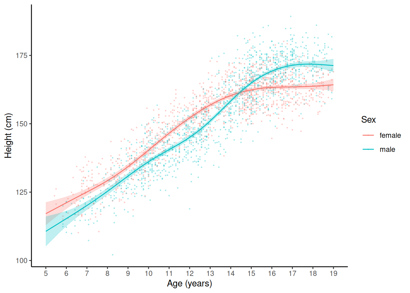
The scam package can be used to estimate shape-constrained generalized additive models (e.g., monotonic and/or concave or convex).
library(scam)
library(blmeco)
data(anoctua)

m <- scam(PA ~ s(elevation, bs = "cv", m = 2), family = binomial, data = anoctua)

d <- data.frame(elevation = seq(50, 650, length = 100))
d$yhat <- predict(m, newdata = d, type = "response")

p <- ggplot(anoctua, aes(x = elevation, y = PA)) + theme_minimal() +
  geom_rug(data = subset(anoctua, PA == 0), alpha = 0.25, sides = "b") +
  geom_rug(data = subset(anoctua, PA == 1), alpha = 0.25, sides = "t") +
  geom_hline(yintercept = c(0, 1), alpha = 0.5) +
  labs(x = "Elevation (meters)", y = "Probability of Presence") +
  scale_x_continuous(breaks = seq(100, 700, by = 50)) +
  geom_line(aes(y = yhat), data = d)
plot(p)
Example: Multiple explanatory variables can be “smoothed” in a GAM. For example, consider the model \[ E(Y) = \beta_0 + f_1(x_1) + f_2(x_2), \] where \(\beta_0 = 5\), \(f_1(x) = \log(x_1)\), and \(f_2(x_2) = 0.05x_2^2\). But suppose we don’t know the functions \(f_1\) and \(f_2\) but instead estimate them from the data.
set.seed(123)

d <- expand.grid(x1 = seq(1, 5, length = 100), x2 = seq(1, 5, length = 100))
d$y <- with(d, 5 + log(x1) + 0.05 * x2^2 + rnorm(nrow(d)))

m <- gam(y ~ s(x1) + s(x2), data = d)
plot(m, select = 1)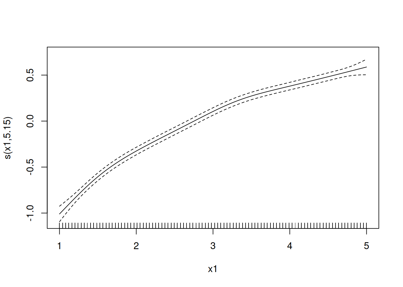
plot(m, select = 2)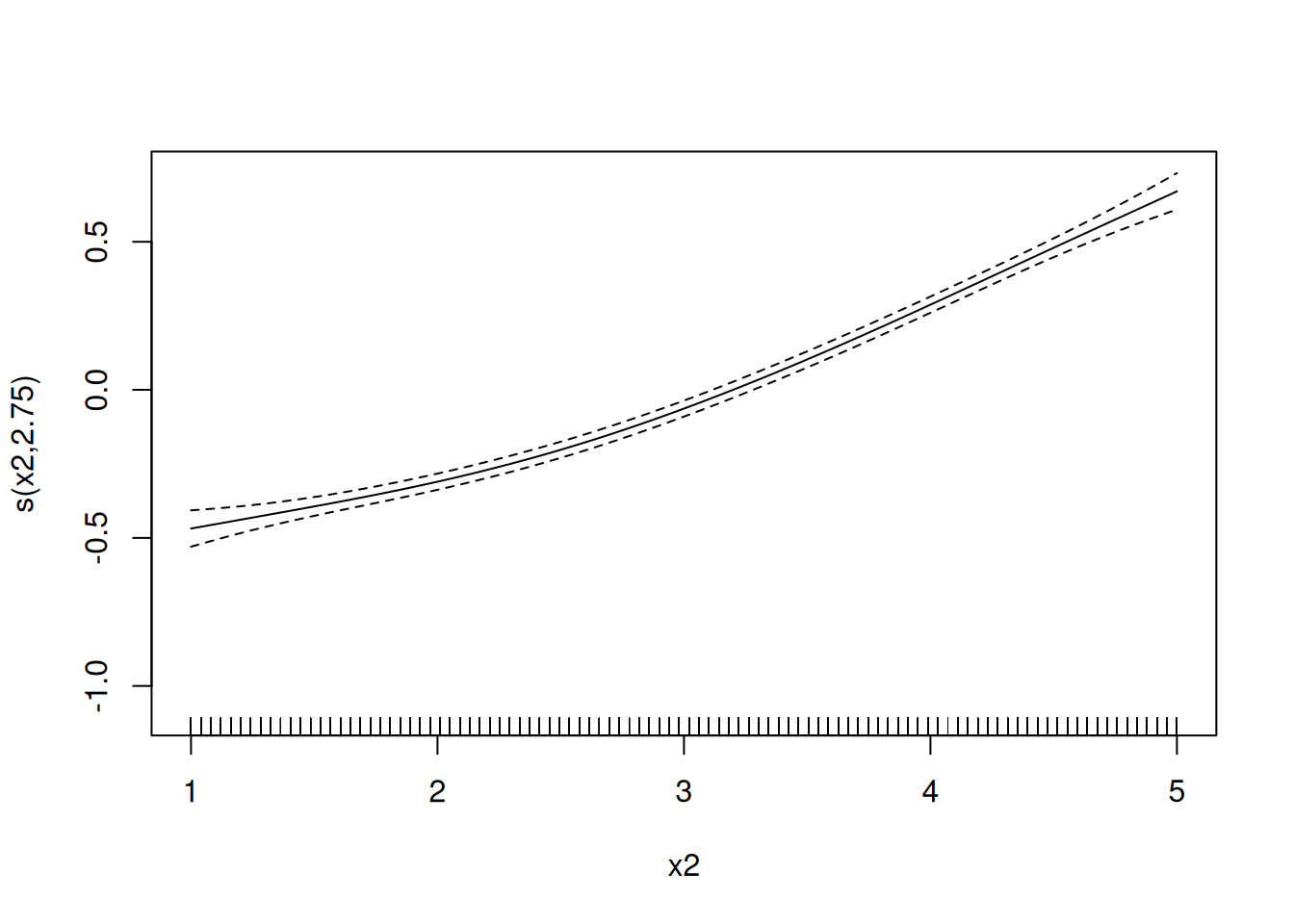 Example: Let’s revisit the crab experiment.
library(Stat2Data)
data(CrabShip)

m <- gam(Oxygen ~ Noise + s(Mass, by = Noise), data = CrabShip)
summary(m)
Family: gaussian
Link function: identity

Formula:
Oxygen ~ Noise + s(Mass, by = Noise)

Parametric coefficients:
            Estimate Std. Error t value Pr(>|t|)
(Intercept)   166.68       8.06   20.67  < 2e-16 ***
Noiseship      74.82      11.47    6.52  3.8e-07 ***
---
Signif. codes:  0 '***' 0.001 '**' 0.01 '*' 0.05 '.' 0.1 ' ' 1

Approximate significance of smooth terms:
                      edf Ref.df     F p-value
s(Mass):Noiseambient 1.45   1.76  4.18   0.054 .
s(Mass):Noiseship    1.54   1.89 15.89 2.4e-05 ***
---
Signif. codes:  0 '***' 0.001 '**' 0.01 '*' 0.05 '.' 0.1 ' ' 1

R-sq.(adj) =  0.685   Deviance explained = 72.3%
GCV =   1276  Scale est. = 1088.8    n = 34
d <- expand.grid(Mass = seq(22, 85, length = 100), Noise = c("ambient","ship"))
d$yhat <- predict(m, newdata = d)
p <- ggplot(CrabShip, aes(x = Mass, y = Oxygen, color = Noise)) +
geom_line(aes(y = yhat), data = d) +
geom_point() + theme_minimal() +
labs(y = "Oxygen Consumption (micromoles/hour)", x = "Mass (g)")
plot(p)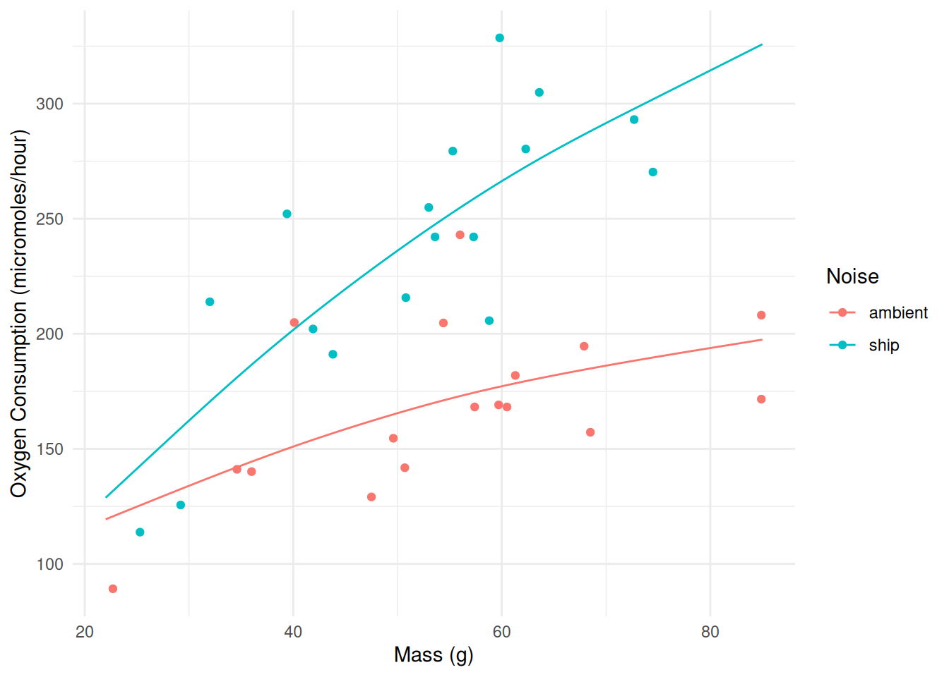
library(emmeans)
pairs(emmeans(m, ~Noise|Mass, at = list(Mass = c(40,50,60))),
  reverse = TRUE, infer = TRUE)
Mass = 40:
contrast estimate SE df lower.CL upper.CL t.ratio p.value
ship - ambient 50.7 16.1 29 17.8 83.6 3.150 0.0037
Mass = 50:
contrast estimate SE df lower.CL upper.CL t.ratio p.value
ship - ambient 70.6 13.5 29 43.0 98.3 5.220 <.0001
Mass = 60:
contrast estimate SE df lower.CL upper.CL t.ratio p.value
ship - ambient 89.1 13.6 29 61.3 117.0 6.550 <.0001
Confidence level used: 0.95 Example: How about the fruit fly data (a GAM ANCOVA)?
library(faraway)
m <- gam(longevity ~ activity + s(thorax), data = fruitfly)
summary(m)
Family: gaussian
Link function: identity

Formula:
longevity ~ activity + s(thorax)

Parametric coefficients:
             Estimate Std. Error t value Pr(>|t|)
(Intercept)     62.04       2.12   29.21  < 2e-16 ***
activityone      2.01       3.01    0.67    0.505
activitylow     -7.34       2.98   -2.46    0.015 *
activitymany     4.03       3.03    1.33    0.186
activityhigh   -20.47       3.03   -6.76  5.8e-10 ***
---
Signif. codes:  0 '***' 0.001 '**' 0.01 '*' 0.05 '.' 0.1 ' ' 1

Approximate significance of smooth terms:
           edf Ref.df    F p-value
s(thorax) 2.86   3.57 32.1  <2e-16 ***
---
Signif. codes:  0 '***' 0.001 '**' 0.01 '*' 0.05 '.' 0.1 ' ' 1

R-sq.(adj) =  0.643   Deviance explained = 66.3%
GCV = 116.92  Scale est. = 109.51    n = 124
d <- expand.grid(activity = levels(fruitfly$activity), thorax = c(0.6,1))
d$yhat <- predict(m, newdata = d, type = "response")
p <- ggplot(fruitfly, aes(x = thorax, y = longevity)) + theme_minimal() +
geom_point() + facet_wrap(~ activity, ncol = 5) +
labs(x = "Thorax Length (mm)", y = "Longevity (days)") +
geom_line(aes(y = yhat), data = d)
plot(p)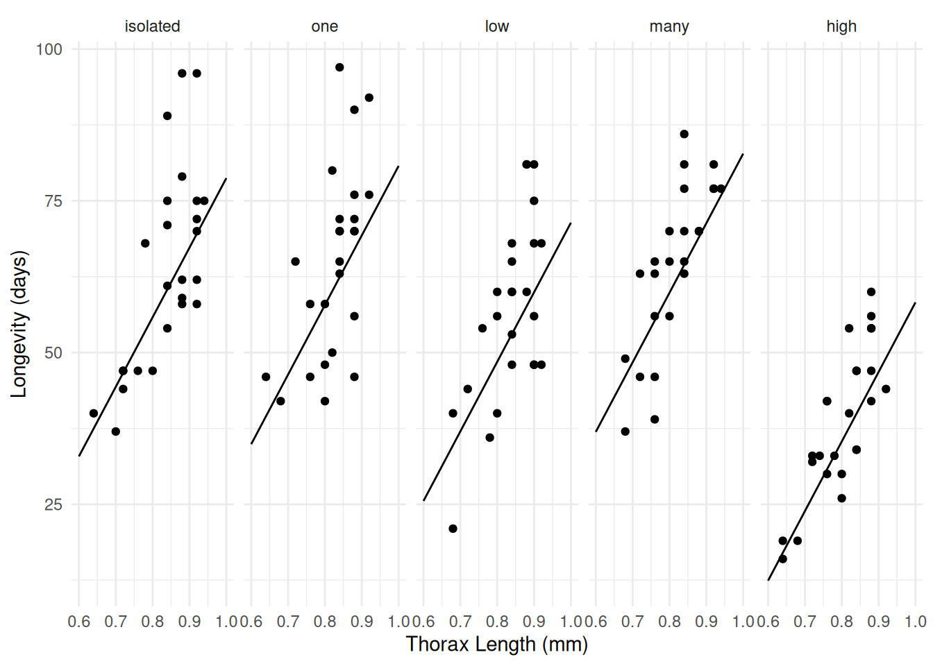 Still fairly linear though!