Monday, April 28
You can also download a PDF copy of this lecture.
Assume that there is a true model \[ Y = f(x) + \epsilon \] where here \(x\) represents one or more explanatory variables, and \(E(\epsilon) = 0\) so that \(E(Y) = f(x)\). But the model we use/assume is \[ Y = g(x) + \tilde\epsilon. \] We use the data to produce \(\hat{g}(x)\), which can be viewed as an estimate of \(f(x)\). Ideally \(\hat{g}(x)\) would tend to be close to \(f(x)\). We can define the expected squared distance between \(\hat{g}(x)\) and \(f(x)\) as the mean squared error \[ E(\hat{g}(x) - f(x))^2, \] which can be decomposed into two terms: \[ E(\hat{g}(x) - f(x))^2 = \underbrace{[E(\hat{g}(x)) - f(x)]^2}_{\text{bias}} + \text{Var}[\hat{g}(x)]. \] A variety of factors will affect the bias and variance.
Different models may be able to produce a \(\hat{g}\) that has higher/lower variance.
As a model becomes more complex the bias tends to decrease, but the variance will tend to increase.
As the sample size increases, the variance will decrease but bias will tend to stay the same, so with large sample sizes we can have more complex models with the same mean squared error.
The design will affect the mean squared error. For example, the “distribution” of the values of the explanatory variable(s) will affect the mean squared error.
For a given design, we would like to select a model such that will minimize \(E(\hat{g}(x) - f(x))^2\) (a bias-variance trade-off). The model should be complex enough to capture the statistical relationship between the response variable and the explanatory variables, but not so complex that it results in “over-fitting” the data.
Prediction Error
The expected prediction error is \(E(Y - \hat{g}(x))^2\) where \(Y\) is a new observation (i.e., one that is not used to obtain \(\hat{g}(x)\)). It can be shown that \[ E(Y - \hat{g}(x))^2 = E(\hat{g}(x) - f(x))^2 + \sigma^2, \] where \(\sigma^2\) is the variance of \(\epsilon\). The choice of model will affect \(E(\hat{g}(x) - f(x))^2\) but not \(\sigma^2\). We can generalize this to multiple values of the explanatory variables and use the expected average prediction error and the expected average mean squared error: \[ E\left(\frac{1}{n}\sum_{i=1}^n (Y_i - \hat{g}(x_i))^2\right) = E\left(\frac{1}{n}\sum_{i=1}^n (\hat{g}(x_i) - f(x_i))^2\right) + \sigma^2. \] Note that minimizing the expected prediction error will therefore minimize the model’s mean squared error. The expected prediction error can be estimated using cross-validation.
Note: Some researchers will use a statistic like the coefficient of determination (i.e., the squared correlation between the predicted and actual values of \(y_i\), sometimes written \(R^2\)) or something similar to estimate (the lack of) prediction error, and to evaluate models. This is not recommended because such estimates can be (very) biased in that they can (severely) underestimate prediction error.
Cross-Validation
An estimate of the expected prediction error is to use \[ \frac{1}{n}\sum_{i=1}^n(y_i - \hat{g}_i(x_i))^2, \] where \(\hat{g}_i\) is the estimate of \(g\) obtained after omitting the \(i\)-th observation. This is sometimes called leave-one-out cross-validation. Another approach is to use \(K\)-fold cross-validation.
Divide the observations randomly into K (nearly) equal sub-samples. Denote these as \(\mathcal{S}_1, \mathcal{S}_2, \dots, \mathcal{S}_K\).
For \(k = 1, 2, \dots, K\), estimate the model without the \(k\)-th sub-sample of observations to obtain \(\hat{g}_k\).
Compute an estimate of the expected prediction error as \[ \frac{1}{n}\sum_{k=1}^K\sum_{i \in \mathcal{S}_k} (y_i - \hat{g}_k(x_i))^2. \]
Comments about K-fold cross-validation:
Leave-one-out cross-validation is a special case where \(K = n\).
The random assignment of observations to sub-samples may need to be constrained somewhat depending on the design (e.g., to avoid empty factor levels).
The process can (and should) be repeated multiple times with different random assignments of observations to sub-samples, and then the estimates are averaged over replications. This reduces the variability of the estimator of the expected prediction error.
The value of K needs to be specified. Values of \(K\) = 5 or \(K\) = 10 are common in practice. Higher values of K result in less bias in the estimation of the expected prediction error, but more variance, and lower values of K result in lower variance but higher bias!
Example: Consider the following data and models.
library(ggplot2)
library(Stat2Data)
data(CrabShip)
p <- ggplot(CrabShip, aes(x = Mass, y = Oxygen, color = Noise)) +
  geom_point() + theme_minimal() +
  labs(y = "Oxygen Consumption (micromoles/hour)", x = "Mass (g)")
plot(p)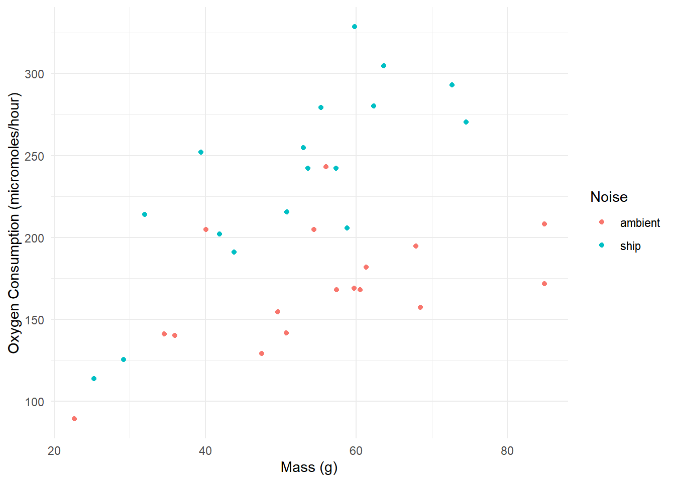
library(dplyr)
m1 <- nls(Oxygen ~ case_when(
  Noise == "ambient" ~ beta_a * Mass^gamma,
  Noise == "ship"    ~ beta_s * Mass^gamma
), start = list(beta_a = 2.9, beta_s = 4.5, gamma = 0.5),
data = CrabShip)
summary(m1)$coefficients
Estimate Std. Error t value Pr(>|t|)
beta_a 17.866 7.571 2.36 2.48e-02
beta_s 26.353 10.922 2.41 2.19e-02
gamma 0.561 0.104 5.41 6.61e-06m2 <- lm(Oxygen ~ -1 + Noise:sqrt(Mass), data = CrabShip)
summary(m2)$coefficients Estimate Std. Error t value Pr(>|t|)
Noiseambient:sqrt(Mass) 22.9 1.09 21.0 2.62e-20
Noiseship:sqrt(Mass) 33.5 1.13 29.8 6.60e-25m3 <- lm(Oxygen ~ -1 + Noise:Mass, data = CrabShip)
summary(m3)$coefficients Estimate Std. Error t value Pr(>|t|)
Noiseambient:Mass 2.91 0.174 16.8 2.09e-17
Noiseship:Mass 4.51 0.187 24.0 4.75e-22m4 <- lm(Oxygen ~ Noise*Mass, data = CrabShip)
summary(m4)$coefficients Estimate Std. Error t value Pr(>|t|)
(Intercept) 103.27 29.389 3.514 0.00142
Noiseship -34.39 43.078 -0.798 0.43096
Mass 1.19 0.512 2.318 0.02746
Noiseship:Mass 2.07 0.783 2.646 0.01286The cvTools package facilitates the cross-validation.
library(cvTools)
set.seed(123)
cv1 <- cvFit(m1, data = CrabShip, y = CrabShip$Oxygen, K = 5, R = 25, cost = mspe)
cv2 <- cvFit(m2, data = CrabShip, y = CrabShip$Oxygen, K = 5, R = 25, cost = mspe)
cv3 <- cvFit(m3, data = CrabShip, y = CrabShip$Oxygen, K = 5, R = 25, cost = mspe)
cv4 <- cvFit(m4, data = CrabShip, y = CrabShip$Oxygen, K = 5, R = 25, cost = mspe)
Here K is the number of folds and R is the
number of repetitions.
cv15-fold CV results:
CV
1257 summary(cv1)5-fold CV results:
CV
Min. 1147
1st Qu. 1174
Median 1226
Mean 1257
3rd Qu. 1335
Max. 1482cvSelect("m1" = cv1, "m2" = cv2, "m3" = cv3, "m4" = cv4)
5-fold CV results:
  Fit   CV
1  m1 1257
2  m2 1171
3  m3 1841
4  m4 1360

Best model:
  CV
"m2"
Akaike’s Information Criterion (AIC)
If maximum likelihood is used to estimate the parameters of a model, we could use the log-likelihood in cross-validation. Imagine we did the following:
Estimate the model parameters with one sample of observations. This produces a log-likelihood function \(\log L\). This is a function of the observations and the estimated parameters.
Compute the value of the log-likelihood function when applying to to a second sample of observations — i.e., compute \(\log L\) with different observations but the same parameter estimates.
A model with a larger expected value of this log-likelihood has a
smaller expected “distance” to the true model (this distance is known as
the Kullback-Leibler distance). An estimate of this expected
log-likelihood is \[
\log L - p,
\] where \(\log L\) is the value
of the maximized log-likelihood function from our data and model, and
\(p\) is the number of estimated
parameters in the model. So we would like to have large values of \(\log L - p\), but for historical reasons we
multiply this by \(-2\) to obtain \[
\text{AIC} = -2\log L + 2p,
\] which we want to be small. If \(n\) is small relative to \(p\) then a better estimator is \[
\text{AIC}_c = \text{AIC} + 2pn/(n-p-1).
\] Example: Consider again the
CrabShip data. We cannot use a mixture of model classes so
we will fit the linear models with nls.
m2 <- nls(Oxygen ~ case_when(
  Noise == "ambient" ~ beta_a * sqrt(Mass),
  Noise == "ship"    ~ beta_s * sqrt(Mass)
), start = list(beta_a = 0, beta_s = 0),
data = CrabShip)

m3 <- nls(Oxygen ~ case_when(
  Noise == "ambient" ~ beta_a * Mass,
  Noise == "ship"    ~ beta_s * Mass
), start = list(beta_a = 0, beta_s = 0),
data = CrabShip)

m4 <- nls(Oxygen ~ case_when(
  Noise == "ambient" ~ alpha_a + beta_a * Mass,
  Noise == "ship"    ~ alpha_s + beta_s * Mass
), start = list(beta_a = 0, beta_s = 0, alpha_a = 0, alpha_s = 0),
data = CrabShip)

library(AICcmodavg)
mynames = c("nonlinear", "-1 + Noise:sqrt(Mass)", "-1 + Noise:Mass", "Noise*Mass")
aictab(list(m1, m2, m3, m4), modnames = mynames)
Model selection based on AICc:

                      K AICc Delta_AICc AICcWt Cum.Wt   LL
-1 + Noise:sqrt(Mass) 3  340       0.00   0.69   0.69 -166
nonlinear             4  342       2.17   0.23   0.92 -166
Noise*Mass            5  344       4.42   0.08   1.00 -166
-1 + Noise:Mass 3 354 14.44 0.00 1.00 -174Example: Consider again our models for the
bliss data.
library(trtools)
m1 <- glm(cbind(dead, exposed - dead) ~ concentration, family = binomial, data = bliss)
m2 <- glm(cbind(dead, exposed - dead) ~ poly(concentration, 2), family = binomial, data = bliss)
m3 <- glm(cbind(dead, exposed - dead) ~ poly(concentration, 3), family = binomial, data = bliss)
m4 <- glm(cbind(dead, exposed - dead) ~ poly(concentration, 4), family = binomial, data = bliss)
AIC can be obtained from summary or using the
AIC function.
summary(m1)
Call:
glm(formula = cbind(dead, exposed - dead) ~ concentration, family = binomial,
    data = bliss)

Coefficients:
              Estimate Std. Error z value Pr(>|z|)
(Intercept)   -14.8084     1.2898   -11.5   <2e-16 ***
concentration   0.2492     0.0214    11.6   <2e-16 ***
---
Signif. codes:  0 '***' 0.001 '**' 0.01 '*' 0.05 '.' 0.1 ' ' 1

(Dispersion parameter for binomial family taken to be 1)

    Null deviance: 289.141  on 15  degrees of freedom
Residual deviance:  12.505  on 14  degrees of freedom
AIC: 58.47

Number of Fisher Scoring iterations: 4AIC(m1)[1] 58.5Utility functions for working with AIC are available in the AICcmodavg package.
library(AICcmodavg)
mynames = c("degree = 1", "degree = 2", "degree = 3", "degree = 4")
aictab(list(m1, m2, m3, m4), modnames = mynames)
Model selection based on AICc:

           K AICc Delta_AICc AICcWt Cum.Wt    LL
degree = 2 3 57.9       0.00   0.60   0.60 -24.9
degree = 1 2 59.4       1.50   0.28   0.89 -27.2
degree = 3 4 61.5       3.59   0.10   0.99 -24.9
degree = 4 5 65.8       7.95   0.01   1.00 -24.9
AIC (or \(\text{AIC}_c\)) is often expressed relative to a candidate model with the lowest AIC by computing the AIC difference defined for the \(k\)-th model as \[ \Delta_k = \text{AIC}_k - \min(\text{AIC}_1,\text{AIC}_2,\dots,\text{AIC}_K) \ge 0. \] These differences are then sometimes normalized into “weights” defined as \[ w_k = \frac{\exp(-\Delta_k/2)}{\exp(-\Delta_1/2) + \exp(-\Delta_2/2) + \cdots + \exp(-\Delta_K/2)}. \] The weights then have the property that \(0 < w_k < 1\) and \(\sum_{k=1}^K w_k = 1\).
Example: Consider an accelerated failure time model for how long it takes for insulating fluids to break down under different constant voltages. What distribution(s) might we specify?
library(Sleuth3)
library(flexsurv)
head(case0802)
Time Voltage Group
1 5.79 26 Group1
2 1579.52 26 Group1
3 2323.70 26 Group1
4 68.85 28 Group2
5 108.29 28 Group2
6 110.29 28 Group2m1 <- flexsurvreg(Surv(Time) ~ Voltage, dist = "gengamma", data = case0802)
m2 <- flexsurvreg(Surv(Time) ~ Voltage, dist = "gamma", data = case0802)
m3 <- flexsurvreg(Surv(Time) ~ Voltage, dist = "weibull", data = case0802)
m4 <- flexsurvreg(Surv(Time) ~ Voltage, dist = "exponential", data = case0802)Most functions in the AICcmodavg have not been
extended to deal with flexsurvreg objects. But we can
compute most quantities of interest “manually” easily enough.
aicc1 <- AIC(m1) + 2*4*76/(76 - 4 - 1) # generalized gamma (p=4)
aicc2 <- AIC(m2) + 2*3*76/(76 - 3 - 1) # gamma (p=3)
aicc3 <- AIC(m3) + 2*3*76/(76 - 3 - 1) # weibull (p=3)
aicc4 <- AIC(m4) + 2*2*76/(76 - 2 - 1) # exponential (p=2)
delta <- c(aicc1,aicc2,aicc3,aicc4) - min(aicc1,aicc2,aicc3,aicc4)
wghts <- exp(-delta/2)/sum(exp(-delta/2))
data.frame(model = c("gengamma","gamma","weibull","exponential"),
  aicc = c(aicc1,aicc2,aicc3,aicc4), delta = delta, weight = wghts)
model aicc delta weight
1 gengamma 617 3.80 0.0834
2 gamma 615 1.22 0.3025
3 weibull 613 0.00 0.5566
4 exponential 618 4.54 0.0575Issues to Consider When Using Prediction Error or AIC
Prediction error and AIC depend on the design. Two design issues to consider are the sample size and the distribution of values of the explanatory variables. Changing the design can change what is the “best” model, even though the underlying “true” model has not changed. Both approaches attempt to identify the best model we can estimate for a given design.
AIC is relative. Unlike simple cross-validation measures it does not give any indication of how well a given model fits the data. The AIC of a model is only interpretable relative to that of another model for the same data.
There is little to no basis for what is a “significant” or “meaningful” difference in an estimate of prediction error or AIC. One reason is that we only have an estimate of the prediction error or the quantity estimated by AIC. Another reason is that to put any weight on a difference in prediction error or AIC we would need to quantify the cost of using a better or worse model.
A complex issue is the effect of model selection on inferences. That is, what is the sampling distribution of a quantity of interest if we first use the data to select a model and then use that model to make inferences. One approach is to use model averaging, but this is not without its own problems.