Wednesday, April 16
You can also download a PDF copy of this lecture.
The Multinomial Logit Model
Recall that a logistic regression model can be written as \[ \log\left[\frac{P(Y_i=1)}{1 - P(Y_i=1)}\right] = \beta_0 + \beta_1 x_{i1} + \dots + \beta_k x_{ik}. \] This can also be written as \[ \log(\pi_{i2}/\pi_{i1}) = \beta_0 + \beta_1 x_{i1} + \dots + \beta_k x_{ik}, \] or \[ \pi_{i2}/\pi_{i1} = e^{\beta_0}e^{\beta_1 x_{i1}} \cdots e^{\beta_k x_{ik}}, \] where \[\begin{align*} \pi_{i2} & = P(Y_i = 1), \\ \pi_{i1} & = P(Y_i = 0). \end{align*}\] Here the ratio of probabilities \(\pi_{i2}/\pi_{i1}\) is the odds that \(Y_i = 1\) rather than \(Y_i = 0\). Note that odds are basically the probability of one event relative to that of another event.
Let \(Y_i = 1, 2, \dots, R\) denote \(R\) categories, but not necessarily ordered in any way, and let \(\pi_{i1}, \pi_{i2}, \dots, \pi_{iR}\) denote the probability of each category. The multinomial logistic regression model can be written as \[\begin{align*} \log(\pi_{i2}/\pi_{i1}) & = \beta_0^{(2)} + \beta_1^{(2)} x_{i1} + \dots + \beta_k^{(2)} x_{ik}, \\ \log(\pi_{i3}/\pi_{i1}) & = \beta_0^{(3)} + \beta_1^{(3)} x_{i1} + \dots + \beta_k^{(3)} x_{ik}, \\ \ & \vdots \\ \log(\pi_{iR}/\pi_{i1}) & = \beta_0^{(R)} + \beta_1^{(R)} x_{i1} + \dots + \beta_k^{(R)} x_{ik}, \end{align*}\] for a system of \(R-1\) equations. This can also be written as \[\begin{align*} \pi_{i2}/\pi_{i1} & = e^{\beta_0^{(2)}}e^{\beta_1^{(2)} x_{i1}} \cdots e^{\beta_k^{(2)} x_{ik}}, \\ \pi_{i3}/\pi_{i1} & = e^{\beta_0^{(3)}}e^{\beta_1^{(3)} x_{i1}} \cdots e^{\beta_k^{(3)} x_{ik}}, \\ \ & \vdots \\ \pi_{iR}/\pi_{i1} & = e^{\beta_0^{(4)}}e^{\beta_1^{(4)} x_{i1}} \cdots e^{\beta_k^{(4)} x_{ik}}, \end{align*}\] so that the model relates the odds of categories 2 through \(R\) relative to the first category (often called a “baseline” or “reference” category). For example, \(\pi_{i3}/\pi_{i1}\) is the odds of the third category versus the first category. Applying the exponential function to a parameter or contrast gives an odds ratio that concerns the change in this odds.
Some algebra shows that the category probabilities can be written as \[\begin{align*} \pi_{i1} & = 1 - (\pi_{i2} + \pi_{i3} + \dots + \pi_{iR}), \\ \pi_{i2} & = \frac{e^{\eta_{i2}}}{1 + e^{\eta_{i2}} + e^{\eta_{i3}} + \dots + e^{\eta_{iR}}} \\ \pi_{i3} & = \frac{e^{\eta_{i3}}}{1 + e^{\eta_{i2}} + e^{\eta_{i3}} + \dots + e^{\eta_{iR}}} \\ \ & \vdots \\ \pi_{iR} & = \frac{e^{\eta_{ir}}}{1 + e^{\eta_{i2}} + e^{\eta_{i3}} + \dots + e^{\eta_{iR}}} \end{align*}\] where \[\begin{align*} \eta_{i2} & = \beta_0^{(2)} + \beta_1^{(2)} x_{i1} + \dots + \beta_k^{(2)} x_{ik}, \\ \eta_{i3} & = \beta_0^{(3)} + \beta_1^{(3)} x_{i1} + \dots + \beta_k^{(3)} x_{ik}, \\ \ & \vdots \\ \eta_{iR} & = \beta_0^{(R)} + \beta_1^{(R)} x_{i1} + \dots + \beta_k^{(R)} x_{ik}. \end{align*}\] We can write this more compactly as \[ \pi_{ic} = \frac{e^{\eta_{ic}}}{1 + \sum_{t=2}^{K} e^{\eta_{it}}} \] or \[ \pi_{ic} = \frac{e^{\eta_{ic}}}{\sum_{t=1}^{K} e^{\eta_{it}}}, \] if we let \(\eta_{i1} = 0\) since \(e^0 = 1\). This is useful for computing and plotting estimated probabilities for each category of the response variable.
Example: Let’s consider again the
pneumo data from the VGAM package.
library(VGAM)
m <- vglm(cbind(normal, mild, severe) ~ exposure.time,
  family = multinomial(refLevel = "normal"), data = pneumo)
summary(m)
Call:
vglm(formula = cbind(normal, mild, severe) ~ exposure.time, family = multinomial(refLevel = "normal"),
    data = pneumo)

Coefficients:
                Estimate Std. Error z value Pr(>|z|)
(Intercept):1    -4.2917     0.5214   -8.23  < 2e-16 ***
(Intercept):2    -5.0598     0.5964   -8.48  < 2e-16 ***
exposure.time:1   0.0836     0.0153    5.47  4.5e-08 ***
exposure.time:2   0.1093     0.0165    6.64  3.2e-11 ***
---
Signif. codes:  0 '***' 0.001 '**' 0.01 '*' 0.05 '.' 0.1 ' ' 1

Names of linear predictors: log(mu[,2]/mu[,1]), log(mu[,3]/mu[,1])

Residual deviance: 13.9 on 12 degrees of freedom

Log-likelihood: -29.5 on 12 degrees of freedom

Number of Fisher scoring iterations: 5

Warning: Hauck-Donner effect detected in the following estimate(s):
'(Intercept):1', '(Intercept):2'


Reference group is level  1  of the response
Note: The categories/levels of the response variable correspond to
the order they are specified in cbind.
Odds ratios can be obtained in the usual way.
exp(cbind(coef(m), confint(m))) 2.5 % 97.5 %
(Intercept):1 0.01368 0.00492 0.0380
(Intercept):2 0.00635 0.00197 0.0204
exposure.time:1 1.08716 1.05508 1.1202
exposure.time:2 1.11548 1.08005 1.1521Here is another nice way to output the parameter estimates.
t(coef(m, matrix = TRUE)) (Intercept) exposure.time
log(mu[,2]/mu[,1]) -4.29 0.0836
log(mu[,3]/mu[,1]) -5.06 0.1093Then we can obtain odds ratio as follows.
exp(t(coef(m, matrix = TRUE))) (Intercept) exposure.time
log(mu[,2]/mu[,1]) 0.01368 1.09
log(mu[,3]/mu[,1]) 0.00635 1.12Plotting the estimated category probabilities can be done as with previous models. First we create a data frame of estimated probabilities by exposure time and category.
d <- data.frame(exposure.time = seq(5, 52, length = 100))
d <- cbind(d, predict(m, newdata = d, type = "response"))
head(d)
exposure.time normal mild severe
1 5.00 0.969 0.0201 0.0106
2 5.47 0.968 0.0209 0.0112
3 5.95 0.967 0.0217 0.0118
4 6.42 0.965 0.0226 0.0124
5 6.90 0.964 0.0235 0.0130
6 7.37 0.962 0.0244 0.0137library(tidyr)
d <- d %>% pivot_longer(cols = c(normal, mild, severe),
names_to = "condition", values_to = "probability")
head(d)# A tibble: 6 × 3
exposure.time condition probability
<dbl> <chr> <dbl>
1 5 normal 0.969
2 5 mild 0.0201
3 5 severe 0.0106
4 5.47 normal 0.968
5 5.47 mild 0.0209
6 5.47 severe 0.0112Next I reorder the factor levels just for aesthetic purposes.
d$condition <- factor(d$condition, levels = c("severe","mild","normal"))And then finally we plot.
p <- ggplot(d, aes(x = exposure.time, y = probability)) +
  geom_line(aes(linetype = condition)) +
  ylim(0, 1) + theme_minimal() +
  labs(x = "Exposure (years)", y = "Probability", linetype = "Condition")
plot(p)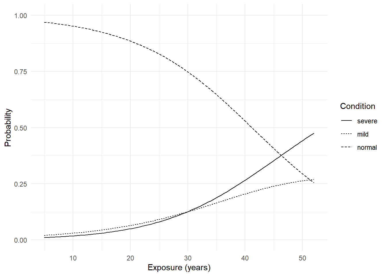
Example: Consider the data frame
alligator from the EffectStars
package.
library(EffectStars)
data(alligator)
head(alligator)
Food Size Gender Lake
1 fish <2.3 male Hancock
2 fish <2.3 male Hancock
3 fish <2.3 male Hancock
4 fish <2.3 male Hancock
5 fish <2.3 male Hancock
6 fish <2.3 male Hancocksummary(alligator) Food Size Gender Lake
bird :13 <2.3:124 female: 89 George :63
fish :94 >2.3: 95 male :130 Hancock :55
invert:61 Oklawaha:48
other :32 Trafford:53
rep :19 For illustration we will just consider just size and gender as explanatory variables.
m <- vglm(Food ~ Gender + Size, data = alligator,
  family = multinomial(refLevel = "bird"))
summary(m)
Call:
vglm(formula = Food ~ Gender + Size, family = multinomial(refLevel = "bird"),
    data = alligator)

Coefficients:
              Estimate Std. Error z value Pr(>|z|)
(Intercept):1   2.0324     0.5204    3.91  9.4e-05 ***
(Intercept):2   1.9897     0.5265    3.78  0.00016 ***
(Intercept):3   1.1748     0.5640    2.08  0.03724 *
(Intercept):4  -0.0526     0.6829   -0.08  0.93859
Gendermale:1    0.6149     0.6338    0.97  0.33197
Gendermale:2    0.5247     0.6589    0.80  0.42585
Gendermale:3    0.4185     0.7030    0.60  0.55162
Gendermale:4    0.5833     0.7841    0.74  0.45691
Size>2.3:1     -0.7535     0.6439   -1.17  0.24193
Size>2.3:2     -1.6746     0.6788   -2.47  0.01362 *
Size>2.3:3     -0.9865     0.7143   -1.38  0.16723
Size>2.3:4      0.1145     0.7962    0.14  0.88565
---
Signif. codes:  0 '***' 0.001 '**' 0.01 '*' 0.05 '.' 0.1 ' ' 1

Names of linear predictors: log(mu[,2]/mu[,1]), log(mu[,3]/mu[,1]), log(mu[,4]/mu[,1]),
log(mu[,5]/mu[,1])

Residual deviance: 588 on 864 degrees of freedom

Log-likelihood: -294 on 864 degrees of freedom

Number of Fisher scoring iterations: 5

No Hauck-Donner effect found in any of the estimates


Reference group is level  1  of the response
To help interpret the output let’s check the level order.
levels(alligator$Food)[1] "bird" "fish" "invert" "other" "rep" Extract parameter estimates and confidence intervals.
cbind(coef(m), confint(m)) 2.5 % 97.5 %
(Intercept):1 2.0324 1.0124 3.052
(Intercept):2 1.9897 0.9577 3.022
(Intercept):3 1.1748 0.0694 2.280
(Intercept):4 -0.0526 -1.3910 1.286
Gendermale:1 0.6149 -0.6273 1.857
Gendermale:2 0.5247 -0.7667 1.816
Gendermale:3 0.4185 -0.9593 1.796
Gendermale:4 0.5833 -0.9535 2.120
Size>2.3:1 -0.7535 -2.0156 0.509
Size>2.3:2 -1.6746 -3.0049 -0.344
Size>2.3:3 -0.9865 -2.3864 0.413
Size>2.3:4 0.1145 -1.4460 1.675t(coef(m, matrix = TRUE)) (Intercept) Gendermale Size>2.3
log(mu[,2]/mu[,1]) 2.0324 0.615 -0.754
log(mu[,3]/mu[,1]) 1.9897 0.525 -1.675
log(mu[,4]/mu[,1]) 1.1748 0.419 -0.986
log(mu[,5]/mu[,1]) -0.0526 0.583 0.114Compute odds ratios.
exp(t(coef(m, matrix = TRUE))) (Intercept) Gendermale Size>2.3
log(mu[,2]/mu[,1]) 7.632 1.85 0.471
log(mu[,3]/mu[,1]) 7.313 1.69 0.187
log(mu[,4]/mu[,1]) 3.237 1.52 0.373
log(mu[,5]/mu[,1]) 0.949 1.79 1.121Note that we can change the reference/baseline category. This changes the model parameterization but does not change the estimated probabilities.
Joint tests of the parameters for each explanatory variable can be
conducted (via a likelihood ratio test) using anova.
anova(m)Analysis of Deviance Table (Type II tests)
Model: 'multinomial', 'VGAMcategorical'
Link: 'multilogitlink'
Response: Food
Df Deviance Resid. Df Resid. Dev Pr(>Chi)
Gender 4 1.03 868 589 0.9052
Size 4 14.08 868 602 0.0071 **
---
Signif. codes: 0 '***' 0.001 '**' 0.01 '*' 0.05 '.' 0.1 ' ' 1Note that for other models we should use anova by
specifying a null model, but here the anova function does
that automatically.
Here are the estimated probabilities.
d <- expand.grid(Gender = c("female","male"), Size = c("<2.3",">2.3"))
d <- cbind(d, predict(m, newdata = d, type = "response"))
head(d)
Gender Size bird fish invert other rep
1 female <2.3 0.0497 0.379 0.363 0.161 0.0471
2 male <2.3 0.0293 0.414 0.362 0.144 0.0499
3 female >2.3 0.1214 0.436 0.166 0.147 0.1292
4 male >2.3 0.0730 0.485 0.169 0.134 0.1391library(tidyr)
d <- d %>% pivot_longer(cols = c(bird, fish, invert, other, rep),
names_to = "food", values_to = "probability")
head(d)# A tibble: 6 × 4
Gender Size food probability
<fct> <fct> <chr> <dbl>
1 female <2.3 bird 0.0497
2 female <2.3 fish 0.379
3 female <2.3 invert 0.363
4 female <2.3 other 0.161
5 female <2.3 rep 0.0471
6 male <2.3 bird 0.0293p <- ggplot(d, aes(x = food, y = probability, color = Gender)) + theme_minimal() +
geom_point(position = position_dodge(width = 0.25)) +
facet_wrap(~ Size) + labs(x = "Food", y = "Probability", color = "Gender")
plot(p)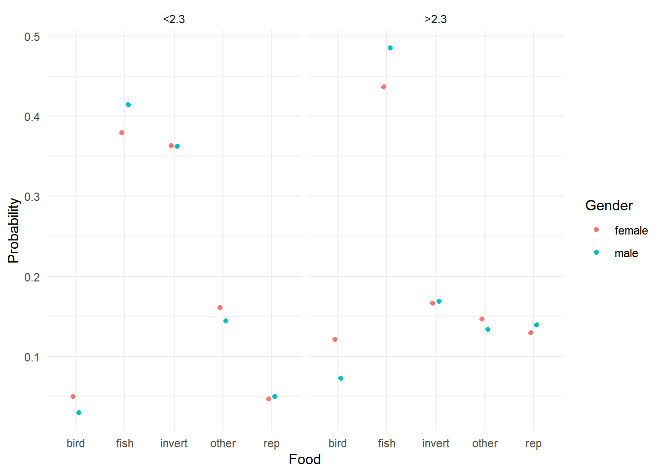
Category-Specific Explanatory Variables
The multinomial logit model can be extended when explanatory
variables vary by response category. For example, consider the
data frame TravelMode from the AER
package.
library(AER)
data(TravelMode)
head(TravelMode, 8)
individual mode choice wait vcost travel gcost income size
1 1 air no 69 59 100 70 35 1
2 1 train no 34 31 372 71 35 1
3 1 bus no 35 25 417 70 35 1
4 1 car yes 0 10 180 30 35 1
5 2 air no 64 58 68 68 30 2
6 2 train no 44 31 354 84 30 2
7 2 bus no 53 25 399 85 30 2
8 2 car yes 0 11 255 50 30 2Here waiting time (wait), vehicle cost
(vcost), and travel time (travel) vary by
travel mode, but household income (income) varies only by
the respondent. For simplicity let’s only consider waiting time and
income as explanatory variables. A multinomial logit model can then be
written as \[\begin{align*}
\log(\pi_{ia}/\pi_{ic}) & = \beta_0^{(a)} + \beta_1
(\text{wait}_i^{(a)} - \text{wait}_i^{(c)}) + \beta_2^{(a)}
\text{income}_i, \\
\log(\pi_{it}/\pi_{ic}) & = \beta_0^{(t)} + \beta_1
(\text{wait}_i^{(t)} - \text{wait}_i^{(c)}) + \beta_2^{(t)}
\text{income}_i, \\
\log(\pi_{ib}/\pi_{ic}) & = \beta_0^{(b)} + \beta_1
(\text{wait}_i^{(b)} - \text{wait}_i^{(c)}) + \beta_2^{(b)}
\text{income}_i. \\
\end{align*}\] If we define \[\begin{align*}
\eta_i^{(a)} & = \beta_0^{(a)} + \beta_1 (\text{wait}_i^{(a)} -
\text{wait}_i^{(c)}) + \beta_2^{(a)} \text{income}_i, \\
\eta_i^{(t)} & = \beta_0^{(t)} + \beta_1 (\text{wait}_i^{(t)} -
\text{wait}_i^{(c)}) + \beta_2^{(t)} \text{income}_i, \\
\eta_i^{(b)} & = \beta_0^{(b)} + \beta_1 (\text{wait}_i^{(b)} -
\text{wait}_i^{(c)}) + \beta_2^{(b)} \text{income}_i,
\end{align*}\] and \(\eta_i^{(c)} =
0\), then we can write the category probabilities as \[\begin{align*}
\pi_{ia} & = \frac{e^{\eta_i^{(a)}}}{e^{\eta_i^{(a)}} +
e^{\eta_i^{(t)}} + e^{\eta_i^{(b)}} + e^{\eta_i^{(c)}}}, \\
\pi_{it} & = \frac{e^{\eta_i^{(t)}}}{e^{\eta_i^{(a)}} +
e^{\eta_i^{(t)}} + e^{\eta_i^{(b)}} + e^{\eta_i^{(c)}}}, \\
\pi_{ib} & = \frac{e^{\eta_i^{(b)}}}{e^{\eta_i^{(a)}} +
e^{\eta_i^{(t)}} + e^{\eta_i^{(b)}} + e^{\eta_i^{(c)}}}, \\
\pi_{ic} & = \frac{e^{\eta_i^{(c)}}}{e^{\eta_i^{(a)}} +
e^{\eta_i^{(t)}} + e^{\eta_i^{(b)}} + e^{\eta_i^{(c)}}}.
\end{align*}\] The quantities \(e^{\eta_i^{(a)}}\), \(e^{\eta_i^{(b)}}\), \(e^{\eta_i^{(b)}}\), and \(e^{\eta_i^{(c)}}\) could be loosely
interpreted as the relative value or “utility” of each response/choice
to the respondent/chooser.
Example: The mlogit function from the
mlogit package will estimate a multinomial logistic
regression model of this type.1
library(mlogit)
m <- mlogit(choice ~ wait | income, reflevel = "car",
  alt.var = "mode", chid.var = "individual", data = TravelMode)
summary(m)
Call:
mlogit(formula = choice ~ wait | income, data = TravelMode, reflevel = "car",
    alt.var = "mode", chid.var = "individual", method = "nr")

Frequencies of alternatives:choice
  car   air train   bus
0.281 0.276 0.300 0.143

nr method
5 iterations, 0h:0m:0s
g'(-H)^-1g = 0.000429
successive function values within tolerance limits

Coefficients :
                  Estimate Std. Error z-value Pr(>|z|)
(Intercept):air    5.98299    0.80797    7.40  1.3e-13 ***
(Intercept):train  5.49392    0.63354    8.67  < 2e-16 ***
(Intercept):bus    4.10653    0.67020    6.13  8.9e-10 ***
wait              -0.09773    0.01053   -9.28  < 2e-16 ***
income:air        -0.00597    0.01151   -0.52    0.604
income:train      -0.06353    0.01367   -4.65  3.4e-06 ***
income:bus        -0.03002    0.01511   -1.99    0.047 *
---
Signif. codes:  0 '***' 0.001 '**' 0.01 '*' 0.05 '.' 0.1 ' ' 1

Log-Likelihood: -192
McFadden R^2:  0.322
Likelihood ratio test : chisq = 183 (p.value = <2e-16)
cbind(coef(m), confint(m)) 2.5 % 97.5 %
(Intercept):air 5.98299 4.3994 7.566578
(Intercept):train 5.49392 4.2522 6.735626
(Intercept):bus 4.10653 2.7929 5.420104
wait -0.09773 -0.1184 -0.077085
income:air -0.00597 -0.0285 0.016593
income:train -0.06353 -0.0903 -0.036731
income:bus -0.03002 -0.0596 -0.000395exp(cbind(coef(m), confint(m))) 2.5 % 97.5 %
(Intercept):air 396.624 81.402 1932.516
(Intercept):train 243.209 70.261 841.871
(Intercept):bus 60.735 16.329 225.903
wait 0.907 0.888 0.926
income:air 0.994 0.972 1.017
income:train 0.938 0.914 0.964
income:bus 0.970 0.942 1.000Example: Here the response variable is the choice of
one of three types of soda. Note that the PoEdata
package must be installed using
remotes::install_github("https://github.com/ccolonescu/PoEdata").
library(dplyr)
library(PoEdata)
data(cola)

mycola <- cola %>% mutate(mode = rep(c("Pepsi","7-Up","Coke"), n()/3)) %>%
   select(id, mode, choice, price, feature, display) %>%
   mutate(feature = factor(feature, levels = 0:1, labels = c("no","yes"))) %>%
   mutate(display = factor(display, levels = 0:1, labels = c("no","yes")))

head(mycola)
id mode choice price feature display
1 1 Pepsi 0 1.79 no no
2 1 7-Up 0 1.79 no no
3 1 Coke 1 1.79 no no
4 2 Pepsi 0 1.79 no no
5 2 7-Up 0 1.79 no no
6 2 Coke 1 0.89 yes yesm <- mlogit(choice ~ price + feature + display | 1, data = mycola,
alt.var = "mode", chid.var = "id")
summary(m)
Call:
mlogit(formula = choice ~ price + feature + display | 1, data = mycola,
    alt.var = "mode", chid.var = "id", method = "nr")

Frequencies of alternatives:choice
 7-Up  Coke Pepsi
0.374 0.280 0.346

nr method
4 iterations, 0h:0m:0s
g'(-H)^-1g = 0.00174
successive function values within tolerance limits

Coefficients :
                  Estimate Std. Error z-value Pr(>|z|)
(Intercept):Coke   -0.0907     0.0640   -1.42   0.1564
(Intercept):Pepsi   0.1934     0.0620    3.12   0.0018 **
price              -1.8492     0.1887   -9.80  < 2e-16 ***
featureyes         -0.0409     0.0831   -0.49   0.6229
displayyes          0.4727     0.0935    5.05  4.3e-07 ***
---
Signif. codes:  0 '***' 0.001 '**' 0.01 '*' 0.05 '.' 0.1 ' ' 1

Log-Likelihood: -1810
McFadden R^2:  0.0891
Likelihood ratio test : chisq = 354 (p.value = <2e-16)
exp(cbind(coef(m), confint(m))) 2.5 % 97.5 %
(Intercept):Coke 0.913 0.806 1.035
(Intercept):Pepsi 1.213 1.075 1.370
price 0.157 0.109 0.228
featureyes 0.960 0.816 1.130
displayyes 1.604 1.336 1.927Example: Consider the following data on choices of two options of traveling by train.
library(mlogit)
data(Train)
head(Train)
id choiceid choice price_A time_A change_A comfort_A price_B time_B change_B comfort_B
1 1 1 A 2400 150 0 1 4000 150 0 1
2 1 2 A 2400 150 0 1 3200 130 0 1
3 1 3 A 2400 115 0 1 4000 115 0 0
4 1 4 B 4000 130 0 1 3200 150 0 0
5 1 5 B 2400 150 0 1 3200 150 0 0
6 1 6 B 4000 115 0 0 2400 130 0 0There are multiple choices for each respondent (id),
which can induce dependencies among the observations, but we will ignore
that here. With only two choices the model reduces to logistic
regression where we use the differences of the properties of
the choices as explanatory variables.
m <- glm(choice == "A" ~ I(price_A - price_B) + I(time_A - time_B),
   family = binomial, data = Train)
summary(m)$coefficients
Estimate Std. Error z value Pr(>|z|)
(Intercept) 0.01874 3.94e-02 0.476 6.34e-01
I(price_A - price_B) -0.00102 5.94e-05 -17.237 1.40e-66
I(time_A - time_B) -0.01397 2.29e-03 -6.106 1.02e-09exp(cbind(coef(m), confint(m))) 2.5 % 97.5 %
(Intercept) 1.019 0.943 1.101
I(price_A - price_B) 0.999 0.999 0.999
I(time_A - time_B) 0.986 0.982 0.991The price is in cents of guilders and the time is in minutes. For interpretation let’s convert the scale of these variables to guilders (equal to 100 cents) and hours (equal to 60 minutes).
m <- glm(choice == "A" ~ I((price_A - price_B)/100) + I((time_A - time_B)/60),
   family = binomial, data = Train)
summary(m)$coefficients
Estimate Std. Error z value Pr(>|z|)
(Intercept) 0.0187 0.03936 0.476 6.34e-01
I((price_A - price_B)/100) -0.1024 0.00594 -17.237 1.40e-66
I((time_A - time_B)/60) -0.8381 0.13725 -6.106 1.02e-09exp(cbind(coef(m), confint(m))) 2.5 % 97.5 %
(Intercept) 1.019 0.943 1.101
I((price_A - price_B)/100) 0.903 0.892 0.913
I((time_A - time_B)/60) 0.433 0.330 0.565Here is how we would estimate this model using mlogit.
The data first need to be reformatted which can be done using the
dfidx function from the mlogit
package.
mytrain <- dfidx(Train, shape = "wide", choice = "choice",
   varying = 4:11, sep = "_")
head(mytrain)
~~~~~~~
first 10 observations out of 5858
~~~~~~~
id choiceid choice price time change comfort idx
1 1 1 TRUE 2400 150 0 1 1:A
2 1 1 FALSE 4000 150 0 1 1:B
3 1 2 TRUE 2400 150 0 1 2:A
4 1 2 FALSE 3200 130 0 1 2:B
5 1 3 TRUE 2400 115 0 1 3:A
6 1 3 FALSE 4000 115 0 0 3:B
7 1 4 FALSE 4000 130 0 1 4:A
8 1 4 TRUE 3200 150 0 0 4:B
9 1 5 FALSE 2400 150 0 1 5:A
10 1 5 TRUE 3200 150 0 0 5:B
~~~ indexes ~~~~
id1 id2
1 1 A
2 1 B
3 2 A
4 2 B
5 3 A
6 3 B
7 4 A
8 4 B
9 5 A
10 5 B
indexes: 1, 2 m <- mlogit(choice ~ I(price/100) + I(time/60) | -1, data = mytrain)
summary(m)
Call:
mlogit(formula = choice ~ I(price/100) + I(time/60) | -1, data = mytrain,
    method = "nr")

Frequencies of alternatives:choice
    A     B
0.503 0.497

nr method
4 iterations, 0h:0m:0s
g'(-H)^-1g = 1.86E-07
gradient close to zero

Coefficients :
             Estimate Std. Error z-value Pr(>|z|)
I(price/100) -0.10235    0.00594   -17.2  < 2e-16 ***
I(time/60)   -0.83684    0.13722    -6.1  1.1e-09 ***
---
Signif. codes:  0 '***' 0.001 '**' 0.01 '*' 0.05 '.' 0.1 ' ' 1

Log-Likelihood: -1850
This model can also be estimated using the
vglmfunction from the VGAM package, although the syntax is very different.↩︎