Wednesday, March 26

Logit Link Function

Let $Y$ be a proportion or binary response variable. The logit link function is defined as $$g[E(Y)] = \log\left[\frac{E(Y)}{1-E(Y)}\right],$$ which implies the mean structure $$E(Y) = \frac{e^{\eta}}{1+e^{\eta}}.$$ Properties:

1. “Symmetric” in the sense that $g(z) = -g(1-z)$. Whether we model the probability of one event or the other is only a choice of parameterization.

2. Allows (easy) use of odds ratios.

3. Connects logistic regression to a variety of models (e.g., multinomial regression) and designs (e.g., case-control studies).

Known as logit in functions like glm. The inverse function $e^z/(1 + e^z)$ is known to R as plogis. This is the default link function for the binomial family.

Example: It is useful to note the “symmetry” of the model in that we can model either the event or its complement.

library(trtools) # for bliss data

# modeling the probability of beetle death
m <- glm(cbind(dead, exposed - dead) ~ concentration, 
  family = binomial(link = logit), data = bliss)
summary(m)$coefficients

              Estimate Std. Error z value Pr(>|z|)
(Intercept)    -14.808     1.2898   -11.5 1.63e-30
concentration    0.249     0.0214    11.7 2.25e-31

# modeling the probability of beetle survival
m <- glm(cbind(exposed - dead, dead) ~ concentration, 
  family = binomial(link = logit), data = bliss)
summary(m)$coefficients

              Estimate Std. Error z value Pr(>|z|)
(Intercept)     14.808     1.2898    11.5 1.63e-30
concentration   -0.249     0.0214   -11.7 2.25e-31

Complementary Log-Log Link Function

Defined as $$g[E(Y)] = \log[-\log[1-E(Y)]],$$ which implies the mean structure $$E(Y_i) = 1 - e^{-e^{\eta_i}}.$$ Known as cloglog to functions like glm.

Properties:

1. Not symmetric. Approaches 1 faster than 0.

2. Variety of applications in bio-assay, epidemiology, and survival analysis.

3. Can be used when the observed response is assumed to depend on an underlying Poisson-distributed count. Let $Z$ be an unobserved response with a Poisson distribution with mean $e^{\eta}$, and let $$Y_i = \begin{cases} 1, & \text{if $Z > 0$}, \\ 0, & \text{if $Z = 0$}. \end{cases}$$ Because $$P(Z = z) = \frac{\lambda^z e^{-\lambda}}{z!}$$ then $$P(Y = 1) = 1 - P(Z = 0) = 1 - e^{-\lambda}.$$ Assuming a Poisson regression model such that $\eta = \exp(\beta_0 + \beta_1 x_1 + \cdots + \beta_k x_k)$ then $$P(Y = 1) = 1 - e^{-e^{\eta}}.$$

   Example: Suppose have the Poisson regression model $$E(Z_i) = \exp(\beta_0 + \beta_1 x_i),$$ but we only observe if the count is greater than zero so what we observe is the binary response $$Y_i = \begin{cases} 1, & \text{if $Z_i > 0$}, \\ 0, & \text{if $Z_i = 0$}. \end{cases}$$ We can make inferences concerning this model using $Y_i$ in a binomial regression model with the complementary log-log link function.

   set.seed(123) # to reproduce results
   n <- 1000 # sample size
   b0 <- 0 
   b1 <- 1 
   
   # simulate data
   d <- data.frame(x = seq(-2, 2, length = n))
   d$z <- rpois(n, lambda = exp(b0 + b1*d$x))
   
   # Poisson regression
   m <- glm(z ~ x, family = poisson, data = d)
   cbind(summary(m)$coefficients, confint(m))

               Estimate Std. Error z value  Pr(>|z|)   2.5 % 97.5 %
   (Intercept)  0.00072     0.0382  0.0188  9.85e-01 -0.0754 0.0745
   x            0.99244     0.0281 35.3029 5.31e-273  0.9379 1.0481

   d$y <- ifelse(d$z > 0, 1, 0) # create binary response
   
   # binomial regression with complementary log-log link function
   m <- glm(y ~ x, family = binomial(link = cloglog), data = d)
   cbind(summary(m)$coefficients, confint(m))

               Estimate Std. Error z value Pr(>|z|)  2.5 % 97.5 %
   (Intercept)  -0.0489     0.0520   -0.94 3.47e-01 -0.152 0.0519
   x             0.9987     0.0574   17.40 8.76e-68  0.890 1.1129

   Note the similarities (and differences) in the inferences.

Log-Log Link Function

Defined as $$g[E(Y)] = \log[-\log E(Y)]$$ which implies the mean structure $$E(Y) = e^{-e^{\eta}}.$$ Properties:

1. Not symmetric. Approaches 1 slower than it approaches 0.

2. Not usually available in software, but is available as loglog from the trtools package.

3. Related to the complementary log-log link function in that if the probability of an event occurring is modeled using a complementary log-log link function, then the probability of an event not occurring can be modeled using the log-log link function.

   Example: The following two models are equivalent.

   library(trtools) # for bliss data and loglog link function
   
   m <- glm(cbind(dead, exposed - dead) ~ concentration, 
     family = binomial(link = loglog), data = bliss)
   summary(m)$coefficients

                 Estimate Std. Error z value Pr(>|z|)
   (Intercept)     -9.058     0.7281   -12.4 1.56e-35
   concentration    0.162     0.0127    12.7 3.36e-37

   m <- glm(cbind(exposed - dead, dead) ~ concentration, 
     family = binomial(link = cloglog), data = bliss)
   summary(m)$coefficients

                 Estimate Std. Error z value Pr(>|z|)
   (Intercept)      9.058     0.7281    12.4 1.56e-35
   concentration   -0.162     0.0127   -12.7 3.36e-37

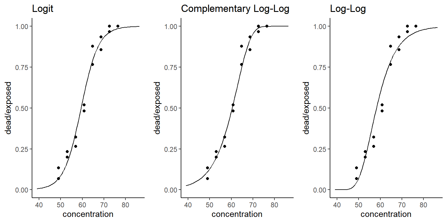
Comparison of Link Functions for Binomial Regression

Example: Consider again the bliss data. The link function is specified through family = binomial(link = X) where X is logit, cloglog, and loglog. Note that we can use these link functions for other “families” such as quasi and quasibinomial.

There are other link functions available in R including probit and cauchit. In theory, there are an infinity of link functions that could be considered. But here we will consider some nicely motivated link functions that have been used in practice.

Natural Response

Logistic regression has the mean structure $$E(Y) = \frac{e^{\eta}}{1 + e^{\eta}},$$ such that $E(Y) \rightarrow 1$ as $\eta \rightarrow \infty$ and $E(Y) \rightarrow 0$ as $\eta \rightarrow -\infty$. And recall that $E(Y)$ is also the probability of the event. In some cases it may not be true that $E(Y) \rightarrow 0$ as $\eta \rightarrow -\infty$.

For simplicity, consider the case where $Y$ is a binary response so that $Y = 0$ or $Y = 1$. Let $N$ be the event that we observe a natural response and $\bar{N}$ the event that we do not observe a natural response. Then $$P(Y = 1) = P(Y = 1|N)P(N) + P(Y = 1|\bar{N})P(\bar{N}) = P(N) + P(Y = 1|\bar{N})P(\bar{N}),$$ noting that $P(Y=1|N) = 1$. If we let $P(N) = \gamma$ and assume that the “non-natural” response follows a logistic regression model so that $$P(Y = 1|\bar{N}) = \frac{e^{\eta}}{1 + e^{\eta}},$$ then $$P(Y = 1) = \gamma + (1-\gamma)\frac{e^{\eta}}{1 + e^{\eta}},$$ noting that $P(\bar{N}) = 1 - P(N) = 1 - \gamma$. In general we can write $$E(Y) = \gamma + (1-\gamma)\frac{e^{\eta}}{1 + e^{\eta}},$$

or $$\log\left[\frac{E(Y)-\gamma}{1 - E(Y)}\right] = \eta.$$ This effectively requires us to modify the link function if $\gamma > 0$. For making inferences we must consider two cases: (1) $\gamma$ is known and can be specified as part of the link function, and (2) $\gamma$ is unknown and must be estimated as an additional parameter. Also note that we can have a natural response variants of other link functions.

Example: Consider again the bliss data. Suppose we know that $\gamma$ = 0.1 (i.e., there is a probability of 0.1 that a beetle will die naturally during the experiment and not due to exposure to carbon disulphide).

m <- glm(cbind(dead, exposed - dead) ~ concentration, 
  data = bliss, family = binomial)
summary(m)$coefficients

              Estimate Std. Error z value Pr(>|z|)
(Intercept)    -14.808     1.2898   -11.5 1.63e-30
concentration    0.249     0.0214    11.7 2.25e-31

Using the natural response link function sometimes requires starting values. An easy way to specify them is to take estimates when using the logit link function.

m.nr <- glm(cbind(dead, exposed - dead) ~ concentration, data = bliss, 
  family = binomial(link = logitnr(0.1)), start = c(-14.8, 0.25))
summary(m.nr)$coefficients

              Estimate Std. Error z value Pr(>|z|)
(Intercept)    -19.128      2.123   -9.01 2.03e-19
concentration    0.314      0.034    9.22 2.98e-20

Note that logitnr is from the trtools package. The interpretation of an odds ratio for this model would be for the odds of death due to carbon disulphide (rather than “natural causes”).

d <- data.frame(concentration = seq(40, 80, length = 100))
d$yhat <- predict(m, newdata = d, type = "response")
d$yhat.nr <- predict(m.nr, newdata = d, type = "response")

p <- ggplot(bliss, aes(x = concentration, y = dead/exposed)) + 
  geom_point() + ylim(0,1) + labs(x = "Concentration", y = "Proportion") + 
  geom_line(aes(y = yhat), data = d) + theme_classic() + 
  geom_line(aes(y = yhat.nr), data = d, linetype = 2) + 
  geom_hline(yintercept = 0.1, color = grey(0.5))
plot(p)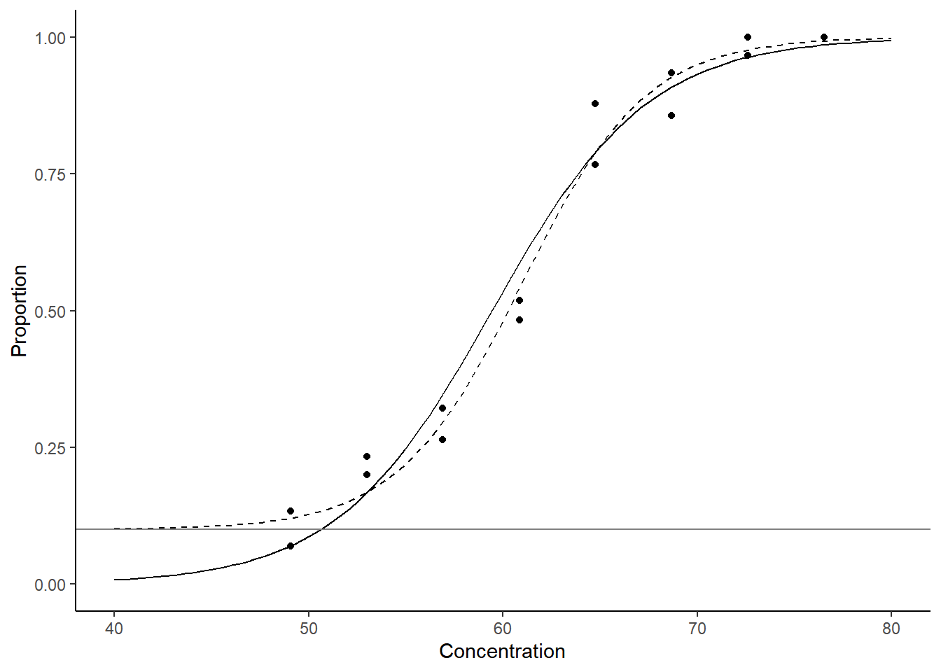

When $\gamma$ is unknown the model is no longer a traditional GLM because there is an unknown parameter in the link function. But we can make inferences using maximum likelihood. This requires a bit of programming.

Example: Consider again the bliss data and model with the logit link function with a natural response. The log-likelihood function is $$\log L = \sum_{i=1}^n \log \left[\frac{m_i!}{r_i!(m_i-r_i)!}p_i^{r_i}(1-p_i)^{m_i-r_i}\right]$$ where $$p_i = \gamma + (1 - \gamma)\frac{e^{\eta_i}}{1 + e^{\eta_i}} \ \ \text{and} \ \ \eta_i = \beta_0 + \beta_1 d_i,$$ where $d_i$ is dose.

We can program the negative log-likelihood function.

nloglik <- function(beta0, beta1, gamma) {
  eta <- beta0 + beta1 * concentration
  prb <- gamma + (1 - gamma) * plogis(eta)
  return(-sum(dbinom(dead, exposed, prb, log = TRUE)))
}

Now we can use another function (mle2) that will solve the maximization (minimization) problem.

library(bbmle)

Warning: package 'bbmle' was built under R version 4.4.3

m <- mle2(nloglik, data = bliss, method = "L-BFGS-B",
  start = list(beta0 = -15, beta1 = 0.25, gamma = 0.1),
  lower = list(beta0 = -Inf, beta1 = -Inf, gamma = 0),
  upper = list(beta0 =  Inf, beta1 =  Inf, gamma = 1))
summary(m)

Maximum likelihood estimation

Call:
mle2(minuslogl = nloglik, start = list(beta0 = -15, beta1 = 0.25, 
    gamma = 0.1), method = "L-BFGS-B", data = bliss, lower = list(beta0 = -Inf, 
    beta1 = -Inf, gamma = 0), upper = list(beta0 = Inf, beta1 = Inf, 
    gamma = 1))

Coefficients:
      Estimate Std. Error z value Pr(z)    
beta0 -19.6470     3.1590   -6.22 5e-10 ***
beta1   0.3214     0.0487    6.60 4e-11 ***
gamma   0.1115     0.0495    2.25 0.024 *  
---
Signif. codes:  0 '***' 0.001 '**' 0.01 '*' 0.05 '.' 0.1 ' ' 1

-2 log L: 50.5 

trtools::lincon(m, a = c(0,1,0), tf = exp, fest = coef, fcov = vcov) # odds ratio

          estimate lower upper
(0,1,0),0     1.38  1.25  1.52

We can also consider a variation on the “natural response” link function where the upper asymptote is $\delta < 1$, or both lower and upper asymptotes of $0 < \gamma < \delta < 1$. The model is then $$E(Y) = \gamma + (\delta - \gamma)\frac{e^{\eta}}{1 + e^{\eta}}.$$ A model with just an upper asymptote of $\delta < 1$ would be $$E(Y) = \delta\frac{e^{\eta}}{1 + e^{\eta}}.$$ An example of an application with an upper asymptote of $\delta$ < 0 might be seed germination (some seeds are “duds” and will never germinate). In the trtools package there is a link function called logitnnr which works like logitnr except it specifies an upper asymptote of $\delta < 0$.

Log Link Function for Binomial Regression

Using a log link function for binomial regression allows us to interpret exponentiated parameters/contrasts in terms of risk ratios (i.e., ratios of probabilities) instead of odds ratios.

Example: Consider the aflatoxicol study.

library(Sleuth3)
p <- ggplot(ex2116, aes(x = Dose, y = Tumor/Total)) + 
   geom_point(alpha = 0.5) + theme_classic() + ylim(0, 1) + 
   labs(x = "Dose (ppm)", y = "Proportion of Trout With Liver Tumors")
plot(p)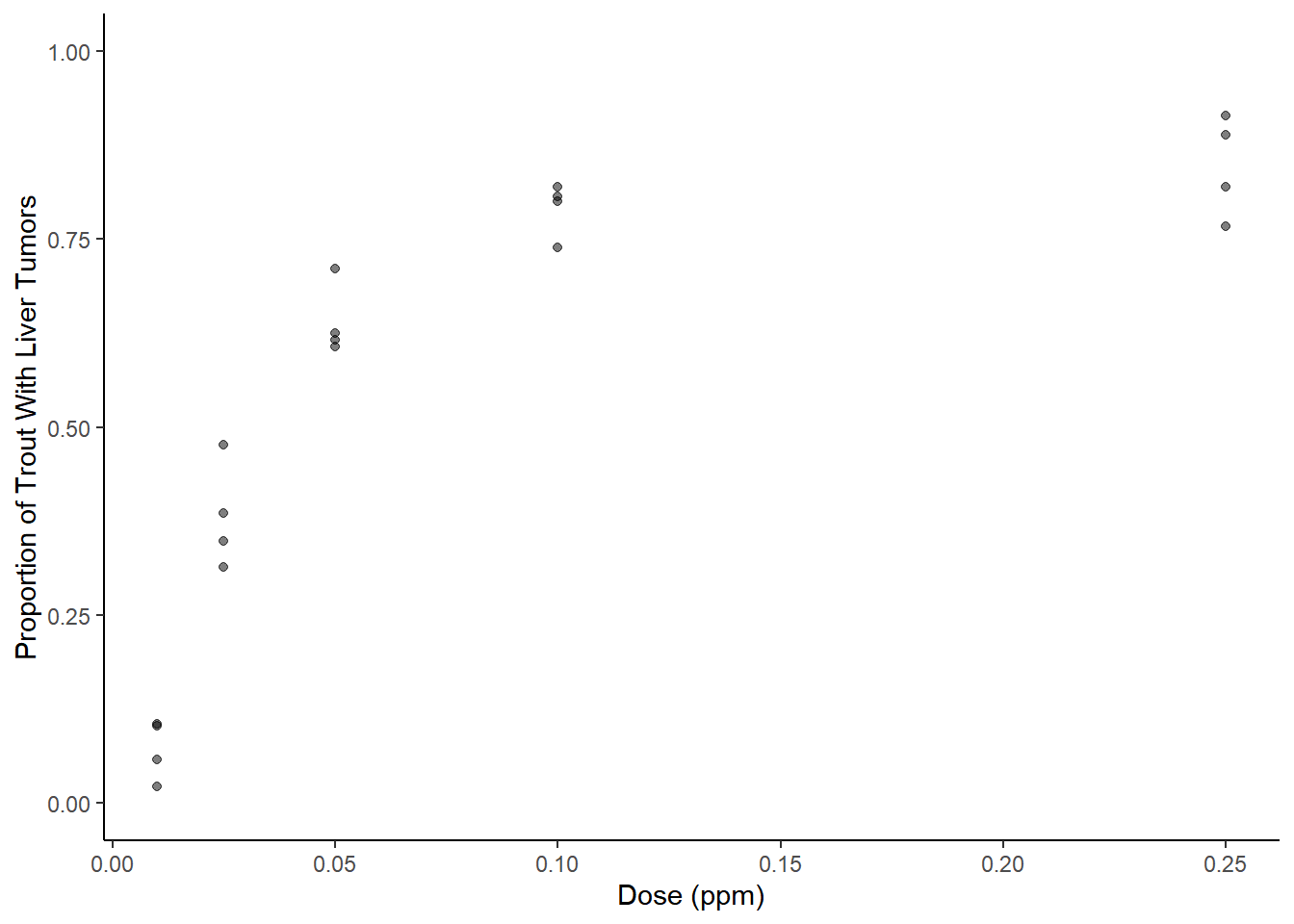

Here we will treat dose as a factor. With the logit link function we can make inferences using odds ratios.

m <- glm(cbind(Tumor, Total - Tumor) ~ factor(Dose), 
  family = binomial(link = logit), data = ex2116)
trtools::contrast(m, tf = exp,
  a = list(Dose = c(0.025,0.05,0.1,0.25)),
  b = list(Dose = 0.01),
  cnames = paste(c(0.025,0.05,0.1,0.25), "vs 0.01"))

              estimate lower upper
0.025 vs 0.01     7.94  5.01  12.6
0.05 vs 0.01     22.92 14.45  36.4
0.1 vs 0.01      48.91 30.24  79.1
0.25 vs 0.01     70.84 42.84 117.1

But using a log link gives us risk ratios.

m <- glm(cbind(Tumor, Total - Tumor) ~ factor(Dose), 
  family = binomial(link = log), data = ex2116)
trtools::contrast(m, tf = exp,
  a = list(Dose = c(0.025,0.05,0.1,0.25)),
  b = list(Dose = 0.01),
  cnames = paste(c(0.025,0.05,0.1,0.25), "vs 0.01"))

              estimate lower upper
0.025 vs 0.01     5.30  3.55  7.91
0.05 vs 0.01      8.89  6.04 13.07
0.1 vs 0.01      10.99  7.50 16.09
0.25 vs 0.01     11.74  8.03 17.18

But be careful using the log link function with binomial regression, particularly with quantitative explanatory variables. It can produce estimated “probabilities” outside $(0,1)$.

Specialty Link Functions for Binomial Regression

library(dplyr)
set.seed(123)

b0 <- 2
b1 <- 1

d <- data.frame(x = seq(0, 3, length = 1000)) %>%
  mutate(days = sample(1:10, n(), replace = TRUE)) %>% 
  mutate(y = rbinom(n(), 1, plogis(b0 + b1*x)^days))
head(d)

        x days y
1 0.00000    3 1
2 0.00300    3 1
3 0.00601   10 0
4 0.00901    2 0
5 0.01201    6 1
6 0.01502    5 0

library(trtools) # for logitexp link function
m <- glm(y ~ x, family = binomial(link = logitexp(exposure = d$days)), data = d)
cbind(summary(m)$coefficients, confint(m))

            Estimate Std. Error z value Pr(>|z|) 2.5 % 97.5 %
(Intercept)     1.90       0.12    15.8 2.40e-56 1.662   2.13
x               1.04       0.10    10.3 4.32e-25 0.844   1.24

library(dplyr)
set.seed(123)

d <- data.frame(m = sample(c(25,50,100,400), 100, replace = TRUE)) %>% 
  mutate(x = seq(-2, 2, length = n())) %>% 
  mutate(z = rbinom(n(), m, plogis(-5 + x/5)))
head(d)

    m     x z
1 100 -2.00 0
2 100 -1.96 0
3 100 -1.92 0
4  50 -1.88 1
5 100 -1.84 0
6  50 -1.80 1

m <- glm(cbind(z, m - z) ~ x, family = binomial(link = logit), data = d)
summary(m)$coefficients

            Estimate Std. Error z value Pr(>|z|)
(Intercept)   -5.031      0.118  -42.57   0.0000
x              0.244      0.102    2.39   0.0171

d <- d %>% mutate(y = ifelse(z > 0, 1, 0))
head(d)

    m     x z y
1 100 -2.00 0 0
2 100 -1.96 0 0
3 100 -1.92 0 0
4  50 -1.88 1 1
5 100 -1.84 0 0
6  50 -1.80 1 1

library(trtools) # for the logitcomp link function
m <- glm(y ~ x, family = binomial(link = logitcomp(d$m)), data = d)
summary(m)$coefficients

            Estimate Std. Error z value  Pr(>|z|)
(Intercept)   -5.015      0.173 -28.986 9.76e-185
x              0.143      0.148   0.969  3.33e-01

library(dplyr)
set.seed(111)

d <- data.frame(x = seq(-3, 3, length = 1000)) %>%
  mutate(z = rbinom(n(), 1, plogis(x)))
head(d)

      x z
1 -3.00 0
2 -2.99 0
3 -2.99 0
4 -2.98 0
5 -2.98 0
6 -2.97 0

tail(d)

        x z
995  2.97 1
996  2.98 0
997  2.98 1
998  2.99 1
999  2.99 1
1000 3.00 1

m <- glm(z ~ x, family = binomial(link = logit), data = d)
summary(m)$coefficients

            Estimate Std. Error z value Pr(>|z|)
(Intercept)    0.122     0.0826    1.48 1.39e-01
x              1.034     0.0618   16.73 7.47e-63

d <- d %>% 
  mutate(y = rbinom(n(), 1, ifelse(z == 1, 0.8, 1 - 0.9)))
head(d)

      x z y
1 -3.00 0 1
2 -2.99 0 0
3 -2.99 0 0
4 -2.98 0 0
5 -2.98 0 0
6 -2.97 0 0

tail(d)

        x z y
995  2.97 1 1
996  2.98 0 0
997  2.98 1 1
998  2.99 1 0
999  2.99 1 1
1000 3.00 1 1

library(trtools) # for logiterr link function
m <- glm(y ~ x, family = binomial(link = logiterr(0.8,0.9)), data = d)
summary(m)$coefficients

            Estimate Std. Error z value Pr(>|z|)
(Intercept)   0.0844      0.127   0.663 5.07e-01
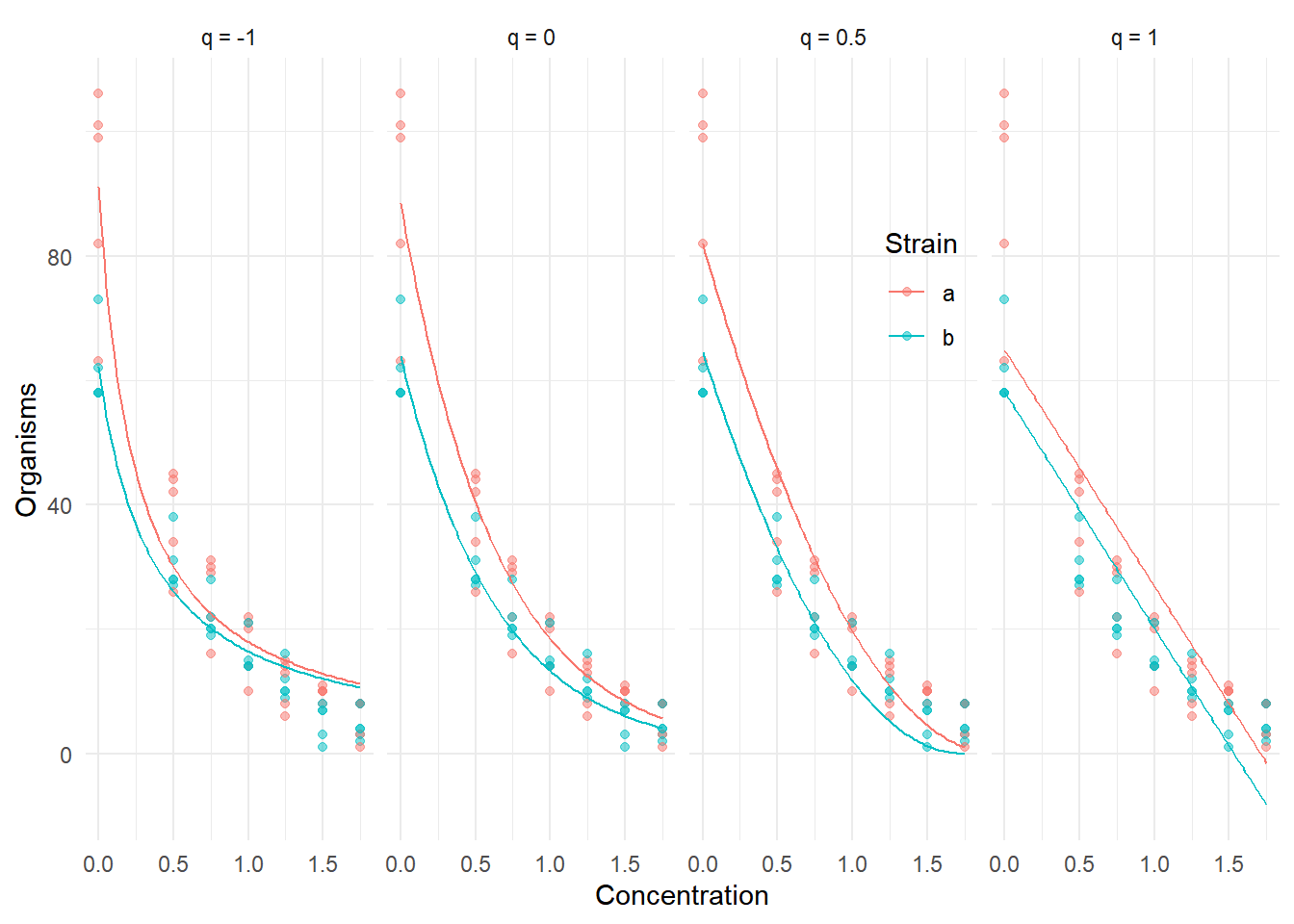
x             0.9658      0.106   9.083 1.06e-19