You can also download a PDF copy
of this lecture.
Marginal Means
A marginal mean is effectively an average of expected
responses. The emmeans package is particularly useful
for making inferences about marginal means. It can also be done using
contrast but it is not a documented feature.
library(trtools)
library(emmeans)
Welcome to emmeans.
Caution: You lose important information if you filter this package's results.
See '? untidy'
Attaching package: 'emmeans'
The following objects are masked from 'package:trtools':

    contrast, neuralgia
Warning: The emmeans package
contains a function called contrast which is not the same
as the function of the same name in the trtools
package, resulting in a namespace conflict if both packages are loaded.
If you have both packages loaded in a given session, use
trtools::contrast and emmeans::contrast to
refer to a given function.
Example: Consider again the data from the platyfish
study.
m <- lm(Percentage ~ Pair, data = Sleuth3::case0602)
summary(m)$coefficients
            Estimate Std. Error t value  Pr(>|t|)
(Intercept)   56.406      3.864 14.5965 5.208e-24
PairPair2      4.479      5.657  0.7919 4.308e-01
PairPair3      6.023      5.384  1.1187 2.667e-01
PairPair4     10.594      5.657  1.8727 6.485e-02
PairPair5      7.805      6.441  1.2118 2.292e-01
PairPair6      6.929      5.657  1.2250 2.243e-01
We see that there are indicator variables for male pairs 2-6. The
model can be written as \[
E(Y_i) =
\begin{cases}
\beta_0, & \text{if the $i$-th observation was from the first
male pair}, \\
\beta_0 + \beta_1, & \text{if the $i$-th observation was from
the second male pair}, \\
\beta_0 + \beta_2, & \text{if the $i$-th observation was from
the third male pair}, \\
\beta_0 + \beta_3, & \text{if the $i$-th observation was from
the fourth male pair}, \\
\beta_0 + \beta_4, & \text{if the $i$-th observation was from
the fifth male pair}, \\
\beta_0 + \beta_5, & \text{if the $i$-th observation was from
the sixth male pair}. \\
\end{cases}
\] We can use contrast to estimate the expected
response for each pair.
trtools::contrast(m, a = list(Pair = paste("Pair", 1:6, sep = "")),
   cnames = paste("Pair", 1:6, sep = ""))
Note how I used a shortcut to specify the pairs.
paste("Pair", 1:6, sep = "")
[1] "Pair1" "Pair2" "Pair3" "Pair4" "Pair5" "Pair6"
This can also be done using the emmeans function from
the package emmeans.
library(emmeans)
emmeans(m, ~ Pair)
 Pair  emmean   SE df lower.CL upper.CL
 Pair1   56.4 3.86 78     48.7     64.1
 Pair2   60.9 4.13 78     52.7     69.1
 Pair3   62.4 3.75 78     55.0     69.9
 Pair4   67.0 4.13 78     58.8     75.2
 Pair5   64.2 5.15 78     54.0     74.5
 Pair6   63.3 4.13 78     55.1     71.6

Confidence level used: 0.95
Denote the six expected responses (one for each pair) as \[\begin{align*}
\mu_1 & = \beta_0, \\
\mu_2 & = \beta_0 + \beta_1, \\
\mu_3 & = \beta_0 + \beta_2, \\
\mu_4 & = \beta_0 + \beta_3, \\
\mu_5 & = \beta_0 + \beta_4, \\
\mu_6 & = \beta_0 + \beta_5.
\end{align*}\] One marginal mean would be the average expected
response across the pairs. This could be written as \[
\mu = \frac{\mu_1 + \mu_2 + \mu_3 + \mu_4 + \mu_5 + \mu_6}{6} =
\beta_0 + \tfrac{1}{6}\beta_1 + \tfrac{1}{6}\beta_2 +
\tfrac{1}{6}\beta_3 + \tfrac{1}{6}\beta_4 + \tfrac{1}{6}\beta_5.
\] We can estimate this quantity with lincon.
lincon(m, a = c(1,1/6,1/6,1/6,1/6,1/6))
                          estimate    se lower upper tvalue df    pvalue
(1,1/6,1/6,1/6,1/6,1/6),0    62.38 1.722 58.95 65.81  36.23 78 1.501e-50
We can also use emmeans.
emmeans(m, ~ 1)
 1       emmean   SE df lower.CL upper.CL
 overall   62.4 1.72 78       59     65.8

Results are averaged over the levels of: Pair
Confidence level used: 0.95
Note that we can use the confidence interval to test the null
hypothesis that \(\mu\) = 50. For a
test statistic and p-value for this test we could write this as \[
\mu = 50 \Leftrightarrow \beta_0 + \tfrac{1}{6}\beta_1 +
\tfrac{1}{6}\beta_2 + \tfrac{1}{6}\beta_3 + \tfrac{1}{6}\beta_4 +
\tfrac{1}{6}\beta_5 = 50 \Leftrightarrow \beta_0 + \tfrac{1}{6}\beta_1 +
\tfrac{1}{6}\beta_2 + \tfrac{1}{6}\beta_3 + \tfrac{1}{6}\beta_4 +
\tfrac{1}{6}\beta_5 - 50 = 0.
\] Here is how we can do that with lincon.
lincon(m, a = c(1,1/6,1/6,1/6,1/6,1/6), b = -50)
                            estimate    se lower upper tvalue df    pvalue
(1,1/6,1/6,1/6,1/6,1/6),-50    12.38 1.722  8.95 15.81  7.189 78 3.439e-10
Here is how we do it with emmeans.
emmeans(m, ~ 1, offset = -50, infer = TRUE)
 1       emmean   SE df lower.CL upper.CL t.ratio p.value
 overall   12.4 1.72 78     8.95     15.8   7.189  <.0001

Results are averaged over the levels of: Pair
Confidence level used: 0.95
By not listing an explanatory variable on the right-hand
side of ~, we are asking that emmeans average
over that explanatory variable. Also note that the argument
infer = TRUE makes the emmeans function
provide both confidence intervals as well as tests.
Note: If we just want to know whether or not we
would reject the null hypothesis that \(\mu =
50\) we can also just look at the confidence interval for \(\mu\).
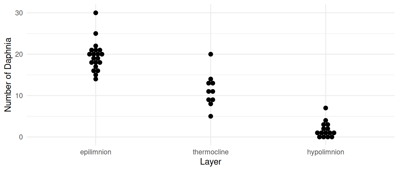
Example: Consider the following data from a survey
of water fleas.
library(ggplot2)
p <- ggplot(daphniastrat, aes(x = layer, y = count)) +
  geom_dotplot(binaxis = "y", stackdir = "center") +
  labs(x = "Layer", y = "Number of Daphnia") + theme_minimal()
plot(p)
 We might model these data using the following linear model.
m <- lm(count ~ layer, data = daphniastrat)
summary(m)$coefficients
                 Estimate Std. Error t value  Pr(>|t|)
(Intercept)         19.50     0.7271  26.820 4.727e-28
layerthermocline    -8.20     1.2593  -6.512 7.293e-08
layerhypolimnion   -17.77     1.1106 -15.997 1.784e-19
So our model can be written as \[
E(Y_i) =
\begin{cases}
\beta_0, & \text{if the $i$-th observation is from the epilimnion
layer}, \\
\beta_0 + \beta_1, & \text{if the $i$-th observation is from the
thermocline layer}, \\
\beta_0 + \beta_2, & \text{if the $i$-th observation is from the
hypolimnion layer}.
\end{cases}
\] Let \(\mu_e\), \(\mu_t\), and \(\mu_h\) denote the expected number of
daphnia per liter for the epilimnion, thermocline, and hypolimnion
layers, respectively (i.e., the density of daphnia in each layer). So
\[
\mu_e = \beta_0, \ \mu_t = \beta_0 + \beta_1, \ \mu_h = \beta_0 +
\beta_2.
\] It is known that the volumes of the epilimnion, thermocline,
and hypolimnion layers are 100, 200, and 400 kL, respectively. The
density for the entire lake is then \[
\mu = \tfrac{100}{700}\mu_e + \tfrac{200}{700}\mu_t +
\tfrac{400}{700}\mu_h =
\beta_0 + \frac{2}{7}\beta_1 + \frac{4}{7}\beta_2.
\] We can estimate this with lincon or
emmeans using the weights option.
lincon(m, a = c(1, 2/7, 4/7))
              estimate    se lower upper tvalue df    pvalue
(1,2/7,4/7),0    7.005 0.572  5.85 8.159  12.25 42 1.907e-15
emmeans(m, ~ 1, weights = c(1/7, 2/7, 4/7))
 1       emmean    SE df lower.CL upper.CL
 overall      7 0.572 42     5.85     8.16

Results are averaged over the levels of: layer
Confidence level used: 0.95
Note that when using emmeans it is important to put the
weights in the correct order. We can verify the order using
level (if the variable is a factor) or by using
weights = "slow.levels".
levels(daphniastrat$layer)
[1] "epilimnion" "thermocline" "hypolimnion"
emmeans(m, ~ 1, weights = "show.levels")
emmeans are obtained by averaging over these factor combinations
        layer
1  epilimnion
2 thermocline
3 hypolimnion
We can estimate the expected number of daphnia per liter for each
layer.
emmeans(m, ~ layer)
 layer       emmean    SE df lower.CL upper.CL
 epilimnion   19.50 0.727 42   18.033    20.97
 thermocline  11.30 1.030 42    9.225    13.38
 hypolimnion   1.73 0.840 42    0.039     3.43

Confidence level used: 0.95
trtools::contrast(m, a = list(layer = c("epilimnion","thermocline","hypolimnion")),
  cnames = c("epilimnion","thermocline","hypolimnion"))
            estimate     se    lower  upper tvalue df    pvalue
epilimnion    19.500 0.7271 18.03274 20.967 26.820 42 4.727e-28
thermocline   11.300 1.0282  9.22498 13.375 10.990 42 6.221e-14
hypolimnion    1.733 0.8395  0.03909  3.428  2.065 42 4.517e-02
We can also do inferences concerning the differences between pairs of
layers.
pairs(emmeans(m, ~ layer), adjust = "none")
 contrast                  estimate   SE df t.ratio p.value
 epilimnion - thermocline      8.20 1.26 42   6.512  <.0001
 epilimnion - hypolimnion     17.77 1.11 42  15.997  <.0001
 thermocline - hypolimnion     9.57 1.33 42   7.207  <.0001
trtools::contrast(m,
  a = list(layer = c("epilimnion","epilimnion","thermocline")),
  b = list(layer = c("thermocline","hypolimnion","hypolimnion")),
  cnames = c("E-T","E-H", "T-H"))
    estimate    se  lower upper tvalue df    pvalue
E-T    8.200 1.259  5.659 10.74  6.512 42 7.293e-08
E-H   17.767 1.111 15.525 20.01 15.997 42 1.784e-19
T-H    9.567 1.327  6.888 12.25  7.207 42 7.363e-09
The adjust = "none" option for pairs
specifies that no adjustment be made to confidence intervals or tests
for the family-wise Type I error rate.
Something to note when using the weights argument with
the emmeans function is that the weights that are used must
sum to one, and if they do not they will be normalized so that they do.
For example, the following provide the same result.
emmeans(m, ~ 1, weights = c(1/7, 2/7, 4/7))
 1       emmean    SE df lower.CL upper.CL
 overall      7 0.572 42     5.85     8.16

Results are averaged over the levels of: layer
Confidence level used: 0.95
emmeans(m, ~ 1, weights = c(1, 2, 4)) # original weights multiplied by 7
 1       emmean    SE df lower.CL upper.CL
 overall      7 0.572 42     5.85     8.16

Results are averaged over the levels of: layer
Confidence level used: 0.95
If you want to use weights that do not sum to one, you can use the
contrast function from the emmeans package
(different from the function of the same name from
trtools).
emmeans(m, ~1, weights = c(1/7, 2/7, 4/7))
 1       emmean    SE df lower.CL upper.CL
 overall      7 0.572 42     5.85     8.16

Results are averaged over the levels of: layer
Confidence level used: 0.95
emmeans::contrast(emmeans(m, ~layer), method = list(layer = c(1/7, 2/7, 4/7)), infer = TRUE)
 contrast estimate    SE df lower.CL upper.CL t.ratio p.value
 layer           7 0.572 42     5.85     8.16  12.245  <.0001

Confidence level used: 0.95
But suppose we wanted to estimate the number of daphnia in
the lake (\(\tau\)). It can be shown
that this is \[
\tau = 700000\mu = 700000\left(\tfrac{1}{7}\mu_e + \tfrac{2}{7}\mu_t +
\tfrac{4}{7}\mu_h\right) = 100000\mu_e + 200000\mu_t + 400000\mu_h.
\] Note that there are 700kL in the lake, which is 700000L (which
is the scale used for the observations). This can be estimated as
follows.
emmeans::contrast(emmeans(m, ~layer),
  method = list(layer = 700000 * c(1/7, 2/7, 4/7)), infer = TRUE)
 contrast estimate    SE df lower.CL upper.CL t.ratio p.value
 layer     4903333 4e+05 42  4095230  5711437  12.245  <.0001

Confidence level used: 0.95
Another approach is to use lincon but your
weights/coefficients will be different since they are applied to \(\beta_0\), \(\beta_1\), and \(\beta_2\).
Marginal Means and “Main Effects”
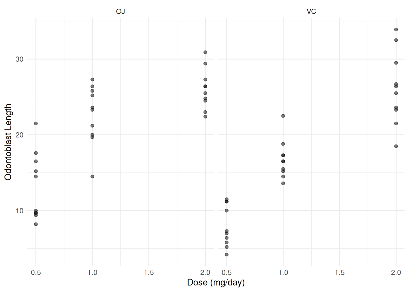
Consider data from a randomized experiment with guinea pigs
administered one of three doses of vitamin C (0.5, 1, or 2 mg/day) via
one of two supplement methods: orange juice (OJ) or ascorbic acid
(VC).
p <- ggplot(ToothGrowth, aes(x = dose, y = len)) +
  geom_point(alpha = 0.5) + facet_wrap(~supp) +
  labs(x = "Dose (mg/day)", y = "Odontoblast Length") + theme_minimal()
plot(p)
 Here we are going to model dose as a categorical variable so we need to
coerce it to a factor. Perhaps the safest approach is to create a new
variable.
Here we are going to model dose as a categorical variable so we need to
coerce it to a factor. Perhaps the safest approach is to create a new
variable.
ToothGrowth$dosef <- factor(ToothGrowth$dose)
Note: Whether a variable is a numeric, a factor, or something else
can be seen use str (for “structure”).
str(ToothGrowth)
'data.frame':   60 obs. of  4 variables:
 $ len  : num  4.2 11.5 7.3 5.8 6.4 10 11.2 11.2 5.2 7 ...
 $ supp : Factor w/ 2 levels "OJ","VC": 2 2 2 2 2 2 2 2 2 2 ...
 $ dose : num  0.5 0.5 0.5 0.5 0.5 0.5 0.5 0.5 0.5 0.5 ...
 $ dosef: Factor w/ 3 levels "0.5","1","2": 1 1 1 1 1 1 1 1 1 1 ...
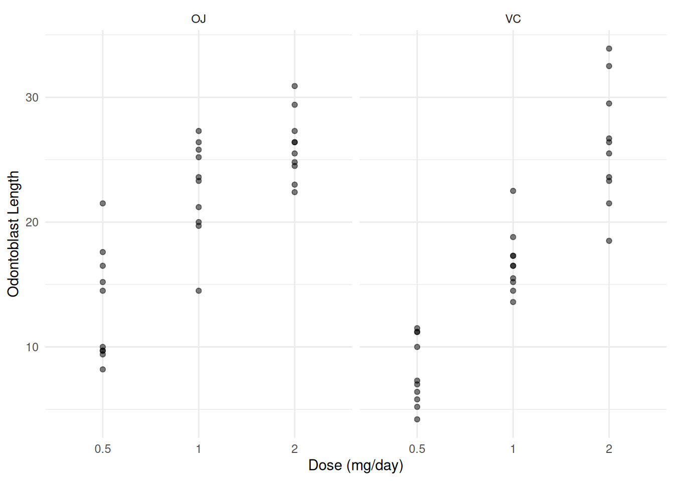
Notice that ggplot responds differently.
summary(ToothGrowth)
      len       supp         dose      dosef
 Min.   : 4.2   OJ:30   Min.   :0.50   0.5:20
 1st Qu.:13.1   VC:30   1st Qu.:0.50   1  :20
 Median :19.2           Median :1.00   2  :20
 Mean   :18.8           Mean   :1.17
 3rd Qu.:25.3           3rd Qu.:2.00
 Max.   :33.9           Max.   :2.00
p <- ggplot(ToothGrowth, aes(x = dosef, y = len)) +
  geom_point(alpha = 0.5) + facet_wrap(~supp) +
  labs(x = "Dose (mg/day)", y = "Odontoblast Length") + theme_minimal()
plot(p)
 Now consider the following linear model.
m <- lm(len ~ dosef + supp + dosef:supp, data = ToothGrowth)
summary(m)$coefficients
              Estimate Std. Error t value  Pr(>|t|)
(Intercept)      13.23      1.148 11.5208 3.603e-16
dosef1            9.47      1.624  5.8312 3.176e-07
dosef2           12.83      1.624  7.9002 1.430e-10
suppVC           -5.25      1.624 -3.2327 2.092e-03
dosef1:suppVC    -0.68      2.297 -0.2961 7.683e-01
dosef2:suppVC     5.33      2.297  2.3207 2.411e-02
The model is \[
E(Y_i) = \beta_0 + \beta_1 x_{i1} + \beta_2 x_{i2} + \beta_3 x_{i3} +
\beta_4 x_{i4} + \beta_5 x_{i5},
\] where \[
x_{i1} =
\begin{cases}
1, & \text{if dose is 1 mg/day}, \\
0, & \text{otherwise},
\end{cases}
\] \[
x_{i2} =
\begin{cases}
1, & \text{if dose is 2 mg/day}, \\
0, & \text{otherwise},
\end{cases}
\] \[
x_{i3} =
\begin{cases}
1, & \text{if supplement type is VC} \\
0, & \text{otherwise},
\end{cases}
\] \[
x_{i4} = x_{i1}x_{i3} =
\begin{cases}
1, & \text{if dose is 1 mg/day and supplement type is VC}, \\
0, & \text{otherwise},
\end{cases}
\] \[
x_{i5} = x_{i2}x_{i3} =
\begin{cases}
1, & \text{if dose is 2 mg/day and supplement type is VC}, \\
0, & \text{otherwise}.
\end{cases}
\]
We can write this model case-wise. \[
E(Y_i) =
\begin{cases}
\beta_0, & \text{if dose is 0.5 mg/day and supplement type is
OJ}, \\
\beta_0 + \beta_1, & \text{if dose is 1 mg/day and supplement
type is OJ}, \\
\beta_0 + \beta_2, & \text{if dose is 2 mg/day and supplement
type is OJ}, \\
\beta_0 + \beta_3, & \text{if dose is 0.5 mg/day and supplement
type is VC}, \\
\beta_0 + \beta_1 + \beta_3 + \beta_4, & \text{if dose is 1
mg/day and supplement type is VC}, \\
\beta_0 + \beta_2 + \beta_3 + \beta_5, & \text{if dose is 2
mg/day and supplement type is VC}. \\
\end{cases}
\] Note that if we omitted the interaction term so that the model
formula is len ~ dosef + supp, then we would have the model
\[
E(Y_i) = \beta_0 + \beta_1 x_{i1} + \beta_2 x_{i2} + \beta_3 x_{i3},
\] which can be written case-wise as \[
E(Y_i) =
\begin{cases}
\beta_0, & \text{if dose is 0.5 mg/day and supplement type is
OJ}, \\
\beta_0 + \beta_1, & \text{if dose is 1 mg/day and supplement
type is OJ}, \\
\beta_0 + \beta_2, & \text{if dose is 2 mg/day and supplement
type is OJ}, \\
\beta_0 + \beta_3, & \text{if dose is 0.5 mg/day and supplement
type is VC}, \\
\beta_0 + \beta_1 + \beta_3 & \text{if dose is 1 mg/day and
supplement type is VC}, \\
\beta_0 + \beta_2 + \beta_3 & \text{if dose is 2 mg/day and
supplement type is VC}. \\
\end{cases}
\]
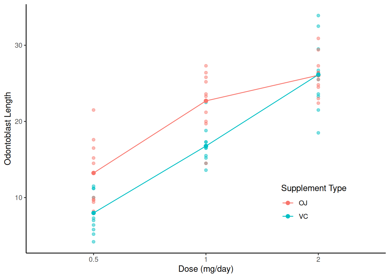
Here is a visualization of the data and the model with the
interaction.
d <- expand.grid(dosef = levels(ToothGrowth$dosef), supp = levels(ToothGrowth$supp))
d$yhat <- predict(m, newdata = d)

p <- ggplot(ToothGrowth, aes(x = dosef, y = len, color = supp)) +
  geom_point(alpha = 0.5) + theme_classic() +
  theme(legend.position = "inside", legend.position.inside = c(0.8,0.2)) +
  geom_point(aes(y = yhat), size = 2, data = d) +
  geom_line(aes(y = yhat, group = supp), data = d) +
  labs(x = "Dose (mg/day)", y = "Odontoblast Length", color = "Supplement Type")
plot(p)
 Consider again the model with the interaction so that \[
E(Y_i) =
\begin{cases}
\beta_0, & \text{if dose is 0.5 mg/day and supplement type is
OJ}, \\
\beta_0 + \beta_1, & \text{if dose is 1 mg/day and supplement
type is OJ}, \\
\beta_0 + \beta_2, & \text{if dose is 2 mg/day and supplement
type is OJ}, \\
\beta_0 + \beta_3, & \text{if dose is 0.5 mg/day and supplement
type is VC}, \\
\beta_0 + \beta_1 + \beta_3 + \beta_4, & \text{if dose is 1
mg/day and supplement type is VC}, \\
\beta_0 + \beta_2 + \beta_3 + \beta_5, & \text{if dose is 2
mg/day and supplement type is VC}. \\
\end{cases}
\] The “cell means” are \[\begin{align}
\mu_{\text{OJ,0.5}} & = \beta_0, \\
\mu_{\text{OJ,1.0}} & = \beta_0 + \beta_1, \\
\mu_{\text{OJ,2.0}} & = \beta_0 + \beta_2, \\
\mu_{\text{VC,0.5}} & = \beta_0 + \beta_3, \\
\mu_{\text{VC,1.0}} & = \beta_0 + \beta_1 + \beta_3 + \beta_4, \\
\mu_{\text{VC,2.0}} & = \beta_0 + \beta_1 + \beta_3 + \beta_5.
\end{align}\] The “marginal means” for supplement type are \[
\mu_{\text{OJ}} = \frac{\mu_{\text{OJ,0.5}} + \mu_{\text{OJ},1.0} +
\mu_{\text{OJ},2.0}}{3} = \beta_0 + \frac{1}{3}\beta_1 +
\frac{1}{3}\beta_2,
\] and \[
\mu_{\text{VC}} = \frac{\mu_{\text{VC,0.5}} + \mu_{\text{VC},1.0} +
\mu_{\text{OJ},2.0}}{3} = \beta_0 + \frac{1}{3}\beta_1 +
\frac{1}{3}\beta_2 + \beta_3 + \frac{1}{3}\beta_4 + \frac{1}{3}\beta_5.
\] We can estimate them using
Consider again the model with the interaction so that \[
E(Y_i) =
\begin{cases}
\beta_0, & \text{if dose is 0.5 mg/day and supplement type is
OJ}, \\
\beta_0 + \beta_1, & \text{if dose is 1 mg/day and supplement
type is OJ}, \\
\beta_0 + \beta_2, & \text{if dose is 2 mg/day and supplement
type is OJ}, \\
\beta_0 + \beta_3, & \text{if dose is 0.5 mg/day and supplement
type is VC}, \\
\beta_0 + \beta_1 + \beta_3 + \beta_4, & \text{if dose is 1
mg/day and supplement type is VC}, \\
\beta_0 + \beta_2 + \beta_3 + \beta_5, & \text{if dose is 2
mg/day and supplement type is VC}. \\
\end{cases}
\] The “cell means” are \[\begin{align}
\mu_{\text{OJ,0.5}} & = \beta_0, \\
\mu_{\text{OJ,1.0}} & = \beta_0 + \beta_1, \\
\mu_{\text{OJ,2.0}} & = \beta_0 + \beta_2, \\
\mu_{\text{VC,0.5}} & = \beta_0 + \beta_3, \\
\mu_{\text{VC,1.0}} & = \beta_0 + \beta_1 + \beta_3 + \beta_4, \\
\mu_{\text{VC,2.0}} & = \beta_0 + \beta_1 + \beta_3 + \beta_5.
\end{align}\] The “marginal means” for supplement type are \[
\mu_{\text{OJ}} = \frac{\mu_{\text{OJ,0.5}} + \mu_{\text{OJ},1.0} +
\mu_{\text{OJ},2.0}}{3} = \beta_0 + \frac{1}{3}\beta_1 +
\frac{1}{3}\beta_2,
\] and \[
\mu_{\text{VC}} = \frac{\mu_{\text{VC,0.5}} + \mu_{\text{VC},1.0} +
\mu_{\text{OJ},2.0}}{3} = \beta_0 + \frac{1}{3}\beta_1 +
\frac{1}{3}\beta_2 + \beta_3 + \frac{1}{3}\beta_4 + \frac{1}{3}\beta_5.
\] We can estimate them using lincon.
lincon(m, a = c(1,1/3,1/3,0,0,0))
                    estimate    se lower upper tvalue df    pvalue
(1,1/3,1/3,0,0,0),0    20.66 0.663 19.33 21.99  31.17 54 3.359e-36
lincon(m, a = c(1,1/3,1/3,1,1/3,1/3))
                        estimate    se lower upper tvalue df    pvalue
(1,1/3,1/3,1,1/3,1/3),0    16.96 0.663 15.63 18.29  25.59 54 7.306e-32
But we can also do it using emmeans.
emmeans(m, ~supp)
 supp emmean    SE df lower.CL upper.CL
 OJ     20.7 0.663 54     19.3     22.0
 VC     17.0 0.663 54     15.6     18.3

Results are averaged over the levels of: dosef
Confidence level used: 0.95
Now suppose we want to estimate the “main effect” which is \[
\mu_{\text{OJ}} - \mu_{\text{VC}} = \frac{\mu_{\text{OJ,0.5}} +
\mu_{\text{OJ},1.0} + \mu_{\text{OJ},2.0}}{3} -
\frac{\mu_{\text{VC,0.5}} + \mu_{\text{VC},1.0} +
\mu_{\text{OJ},2.0}}{3} = -\beta_3 - \frac{1}{3}\beta_4 -
\frac{1}{3}\beta_5.
\] We can do this using lincon.
lincon(m, a = c(0,0,0,-1,-1/3,-1/3))
                       estimate     se lower upper tvalue df    pvalue
(0,0,0,-1,-1/3,-1/3),0      3.7 0.9376  1.82  5.58  3.946 54 0.0002312
But we can also use functions from the emmeans
package.
pairs(emmeans(m, ~supp), infer = TRUE)
 contrast estimate    SE df lower.CL upper.CL t.ratio p.value
 OJ - VC       3.7 0.938 54     1.82     5.58   3.946  0.0002

Results are averaged over the levels of: dosef
Confidence level used: 0.95
The main effect of dose concerns differences among the marginal means
of dose defined as \(\mu_{0.5}\), \(\mu_{1}\) and \(\mu_{2}\) where \[
\mu_{0.5} = \frac{\mu_{\text{OJ},0.5} + \mu_{\text{VC,0.5}}}{2}, \ \
\
\mu_1 = \frac{\mu_{\text{OJ},1} + \mu_{\text{VC,1}}}{2}, \ \ \
\mu_2 = \frac{\mu_{\text{OJ},2} + \mu_{\text{VC,2}}}{2}.
\]
emmeans(m, ~ dosef)
 dosef emmean    SE df lower.CL upper.CL
 0.5     10.6 0.812 54     8.98     12.2
 1       19.7 0.812 54    18.11     21.4
 2       26.1 0.812 54    24.47     27.7

Results are averaged over the levels of: supp
Confidence level used: 0.95
pairs(emmeans(m, ~ dosef), adjust = "none")
 contrast          estimate   SE df t.ratio p.value
 dosef0.5 - dosef1    -9.13 1.15 54  -7.951  <.0001
 dosef0.5 - dosef2   -15.49 1.15 54 -13.493  <.0001
 dosef1 - dosef2      -6.37 1.15 54  -5.543  <.0001

Results are averaged over the levels of: supp
Main Effects in Anova Tables
In ANOVA tables the test of the “main effect” is the (joint) null
hypothesis that all pairwise differences are zero. For the variable dose
the null hypothesis is \(\mu_{0.5} = \mu_{1} =
\mu_{2}\). This can be done using the test
function.
test(pairs(emmeans(m, ~ dosef)), joint = TRUE)
 df1 df2 F.ratio p.value note
   2  54  92.000  <.0001  d

d: df1 reduced due to linear dependence
This is the traditional main effect that is sometimes reported in an
“ANOVA table” such as that produced by Anova from the
car package.
library(car)
m <- lm(len ~ dosef + supp + dosef:supp, data = ToothGrowth,
  contrast = list(dosef = contr.sum, supp = contr.sum))
Anova(m, type = 3)
Anova Table (Type III tests)

Response: len
            Sum Sq Df F value  Pr(>F)
(Intercept)  21236  1 1610.39 < 2e-16 ***
dosef         2426  2   92.00 < 2e-16 ***
supp           205  1   15.57 0.00023 ***
dosef:supp     108  2    4.11 0.02186 *
Residuals      712 54
---
Signif. codes:  0 '***' 0.001 '**' 0.01 '*' 0.05 '.' 0.1 ' ' 1
The option
contrast = list(dosef = contr.sum, supp = contr.sum) is
necessary here for the Anova function to do the correct
calculations.
The test of the main effect of supplement method was given by
pairs(emmeans(m, ~ supp), infer = TRUE)
 contrast estimate    SE df lower.CL upper.CL t.ratio p.value
 OJ - VC       3.7 0.938 54     1.82     5.58   3.946  0.0002

Results are averaged over the levels of: dosef
Confidence level used: 0.95
We do not need a joint test here since there are only two marginal
means, but here it is anyway.
test(pairs(emmeans(m, ~ supp)), joint = TRUE)
 df1 df2 F.ratio p.value
   1  54  15.572  0.0002