Monday, January 27

You can also download a PDF copy of this lecture.

The purpose of this exercise is to familiarize you with the specification of linear models and contrasts within R. You will need to have the following packages installed: abd, cowplot, ggplot2, and trtools. You should already have ggplot2 and trtools installed. The other packages can be installed using install.packages("abd") and install.packages("cowplot"), or install.packages(c("abd","cowplot")).

This exercise features data from a study published in Nature in 2006.¹ The data can be found in the data frame MoleRats, included in the package abd. You can inspect the data frame by typing MoleRats at the prompt after you load the package with library(abd), and you can look at a summary of the data with summary(MoleRats) or the structure of the variables with str(MoleRats). The study concerned two “castes” of Damaraland mole-rats (Cryptomys damarensis): frequent workers (denoted here as “worker”) and infrequent workers (denoted here as “lazy”). The researchers observed the body mass (g) and daily energy expenditure (kJ/day) of samples mole-rats from both castes. Our objective is to model the difference between the two castes in terms of daily energy expenditure. However, mole-rats in the two castes differ by body mass, which may also be related to energy expenditure.

Here are plots of the raw data, showing the distribution of log energy expenditure for lazy and worker caste rats, and then again but also taking into account the (log) mass of the rats.

library(abd)     # for the data
library(ggplot2) # for plotting
library(cowplot) # for use of the plot_grid function

# boxplot
p1 <- ggplot(MoleRats, aes(x = caste, y = ln.energy)) + 
   geom_boxplot() + geom_point() + theme_minimal() + 
   labs(x = "Caste", y = "Log Energy Expenditure (log kJ/Day)")

# scatterplot
p2 <- ggplot(MoleRats, aes(x = ln.mass, y = ln.energy, color = caste)) +
   geom_point() + theme_minimal() + 
  theme(legend.position = "inside", legend.position.inside = c(0.9, 0.2)) +
   labs(x = "Log Mass (log g)", y = NULL, color = "Caste")

# plot both plots side-by-side
plot_grid(p1, p2, align = "h", rel_widths = c(1,3))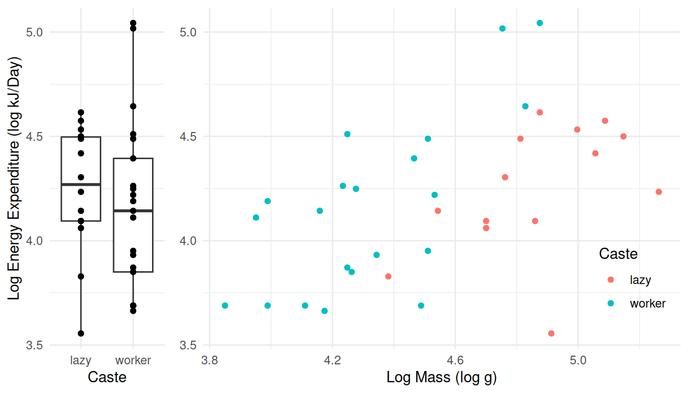

Note that both energy expenditure and mass are recorded on the (natural) log scale. We will be modeling both of these variables on the log scale.

First consider a model where expected log energy expenditure is modeled as a function of only caste. Use the lm function to estimate this model. We should see in the output of the summary function applied to the model object that R will, by default, parameterize this model as \[ E(Y_i) = \beta_0 + \beta_1 d_i, \] where $Y_i$ is the log of energy expenditure of the $i$-th observation and \[ d_i = \begin{cases} 1, & \text{if the $i$-th observation is of a worker}, \\ 0, & \text{otherwise}, \end{cases} \] so that the model can also be written as \[ E(Y_i) = \begin{cases} \beta_0, & \text{if the $i$-th observation is from the lazy caste}, \\ \beta_0 + \beta_1, & \text{if the $i$-th observation is from the worker caste}. \end{cases} \]

Solution: We can estimate the model as follows and confirm the parameterization using the output from summary.
```
m <- lm(ln.energy ~ caste, data = MoleRats)
summary(m)$coefficients
```
```
            Estimate Std. Error t value  Pr(>|t|)
(Intercept)  4.24601     0.1008 42.1150 2.885e-30
casteworker -0.08902     0.1302 -0.6839 4.988e-01
```
The casteworker shows that an indicator variable was created that assumes a value of one for any observation where the caste is worker, and zero otherwise.
Consider the following three quantities and how they can be expressed as functions of the model parameters: the expected log energy expenditure of mole-rats from the lazy caste ($\beta_0$), the expected log energy expenditure of mole-rats from the worker caste ($\beta_0 + \beta_1$), and the difference in expected log energy expenditure between the two castes ($\beta_1$ if we subtract lazy from worker). Note that using summary provides inferences for $\beta_0$ and $\beta_1$, but not $\beta_0 + \beta_1$. All three quantities can be written as a linear combination of the form \[ \ell = a_0\beta_0 + a_1\beta_1 + b. \] How can we use the lincon and contrast functions to estimate these three quantities? Note that inferences for two of these quantities — i.e., the expected log expenditure of mole-rats of the lazy caste and the difference in the expected log expenditures between the two castes — should match those given by using summary and confint applied to the model object.

Solution: First we need to load the trtools package to use lincon and contrast.
```
library(trtools)
```
We can use lincon to produce inferences for $\beta_0$, $\beta_0 + \beta_1$, and $\beta_1$ as follows.
```
lincon(m, a = c(1,0)) # b0
```
```
        estimate     se lower upper tvalue df    pvalue
(1,0),0    4.246 0.1008 4.041 4.451  42.12 33 2.885e-30
```
```
lincon(m, a = c(1,1)) # b0 + b1
```
```
        estimate      se lower upper tvalue df   pvalue
(1,1),0    4.157 0.08232  3.99 4.324   50.5 33 7.89e-33
```
```
lincon(m, a = c(0,1)) # b1
```
```
        estimate     se   lower  upper  tvalue df pvalue
(0,1),0 -0.08902 0.1302 -0.3538 0.1758 -0.6839 33 0.4988
```
Note, however, that single parameter inferences (i.e., $\beta_0$ and $\beta_1$) are also produced by summary. We can produce inferences about the expected response for the two castes using contrast as follows.
```
contrast(m, 
  a = list(caste = c("lazy","worker")),
  cnames = c("lazy","worker"))
```
```
       estimate      se lower upper tvalue df    pvalue
lazy      4.246 0.10082 4.041 4.451  42.12 33 2.885e-30
worker    4.157 0.08232 3.990 4.324  50.50 33 7.890e-33
```
And the following will produce inferences concerning the difference in the expected response between the worker and lazy castes.
```
contrast(m,
  a = list(caste = "worker"),
  b = list(caste = "lazy"))
```
```
 estimate     se   lower  upper  tvalue df pvalue
 -0.08902 0.1302 -0.3538 0.1758 -0.6839 33 0.4988
```
Note that lincon andd contrast produce the same results. Also note that the estimated expected response for the worker caste is slightly less than that for the lazy caste, although the difference is not statistically significant at conventional significance levels.
The model we considered above compares the two castes of mole-rats, but it does not account for differences in their sizes. The lazy mole-rats tend to be larger than the worker mole-rats. It may be useful to compare rats in the two castes while “controlling for size” meaning that comparisons can be made between mole-rats in different castes but of the same size. We can use lm to estimate a linear model that includes both caste and the log of mass as explanatory variables. If we list caste first in the right-hand side of the model formula then the model will be parameterized as \[ E(Y_i) = \beta_0 + \beta_1 d_i + \beta_2 \log(m_i), \] where $d_i$ is defined as before and $\log(m_i)$ is the log of mass of the $i$-th observation (i.e., the ln.mass variable). Note that this model can also be written as \[ E(Y_i) = \begin{cases} \beta_0 + \beta_2 \log(m_i), & \text{if the $i$-th observation is from the lazy caste}, \\ \beta_0 + \beta_1 + \beta_2 \log(m_i), & \text{if the $i$-th observation is from the worker caste}. \end{cases} \] Solution: The model can be estimated as follows.
```
m <- lm(ln.energy ~ caste + ln.mass, data = MoleRats)
summary(m)$coefficients
```
```
            Estimate Std. Error t value  Pr(>|t|)
(Intercept) -0.09687     0.9423 -0.1028 9.188e-01
casteworker  0.39334     0.1461  2.6922 1.120e-02
ln.mass      0.89282     0.1930  4.6252 5.887e-05
```
The parameterization can be confirmed from the output from summary.

Using the code given above, add lines to the plot to show the estimated expected log energy expenditure as a function of log mass and caste.

Solution: First we create a data set to hold estimated expected responses at a variety of values of the explanatory variables.

d <- expand.grid(caste = c("lazy","worker"), ln.mass = seq(3.8, 5.3, length = 100))
d$yhat <- predict(m, newdata = d)

Then we “add to” the plot we created above.

p2 <- p2 + geom_line(aes(y = yhat), data = d)
plot(p2)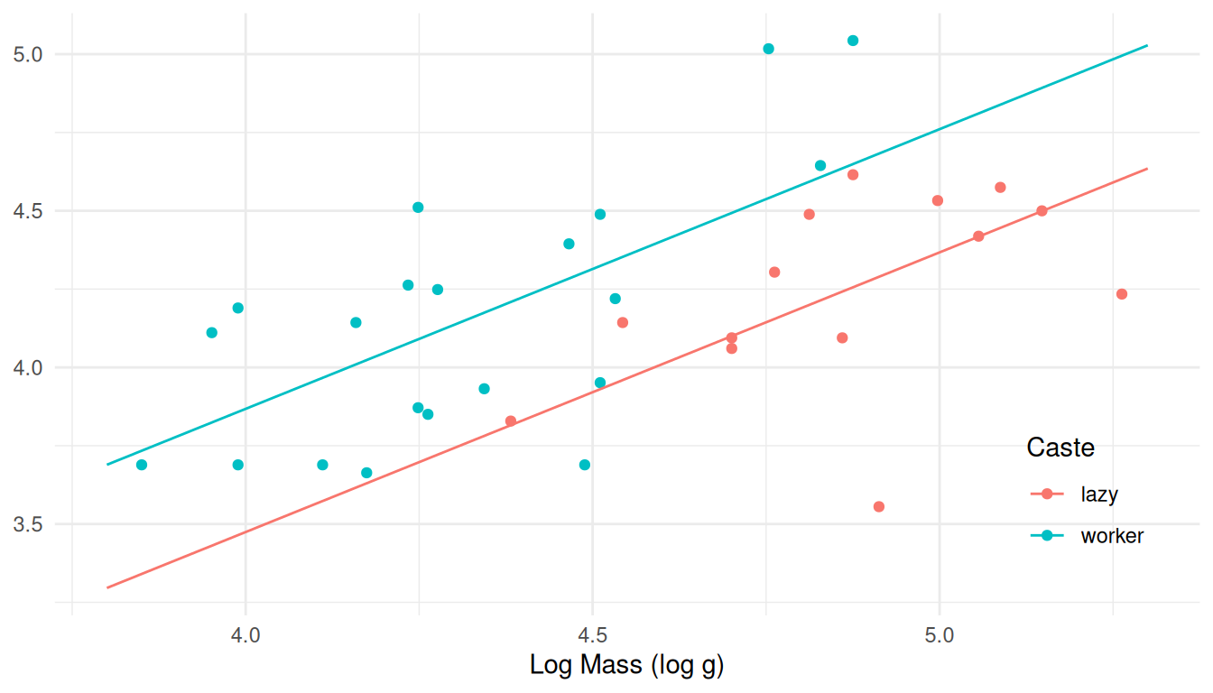

If we had not already created the plot object above then we could do as follows.

p <- ggplot(MoleRats, aes(x = ln.mass, y = ln.energy, color = caste)) +
  geom_point() + theme_minimal() + 
  theme(legend.position = "inside", legend.position.inside = c(0.9, 0.2)) +
  labs(x = "Log Mass (log g)", y = "Log Energy Expenditure (log kJ/Day)", color = "Caste") + 
  geom_line(aes(y = yhat), data = d)
plot(p)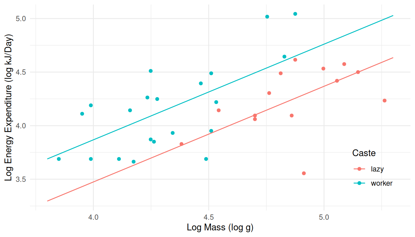

With the model now including the log of mass as an explanatory variable, comparisons between the castes must also consider mass. How can we use contrast to estimate the expected log energy consumption for a mole-rat from each of the two castes with a log mass of 4.5? Also how can we estimate the difference in expected log energy expenditure between the two castes for a mole-rat with log mass 4.5? How can we do the same for log masses of 4.0 and 5.0? Our estimates should be consistent with the figure (i.e., they should look reasonable based on “eyeball” estimates from the figure). Also because the model specifies that the two lines are parallel, the estimated difference in expected log energy consumption between the castes will not depend on mass.

Solution: Here are the estimates of the expected response for a lazy mole-rat at three different masses, and also a worker mole-rat at the same masses.worker
```
contrast(m, a = list(caste = "lazy", ln.mass = c(4,4.5,5)), cnames = c(4,4.5,5))
```
```
    estimate      se lower upper tvalue df    pvalue
4      3.474 0.18470 3.098 3.851  18.81 32 7.300e-19
4.5    3.921 0.10595 3.705 4.137  37.00 32 7.733e-28
5      4.367 0.08348 4.197 4.537  52.31 32 1.426e-32
```
```
contrast(m, a = list(caste = "worker", ln.mass = c(4,4.5,5)), cnames = c(4,4.5,5))
```
```
    estimate      se lower upper tvalue df    pvalue
4      3.868 0.09000 3.684 4.051  42.98 32 7.067e-30
4.5    4.314 0.07309 4.165 4.463  59.02 32 3.120e-34
5      4.761 0.14566 4.464 5.057  32.68 32 3.725e-26
```
And here we make inferences about the difference in the expected response at different values of log mass as follows.
```
contrast(m, 
  a = list(caste = "worker", ln.mass = c(4,4.5,5)),
  b = list(caste = "lazy", ln.mass = c(4,4.5,5)),
  cnames = c(4,4.5,5))
```
```
    estimate     se   lower upper tvalue df pvalue
4     0.3933 0.1461 0.09573 0.691  2.692 32 0.0112
4.5   0.3933 0.1461 0.09573 0.691  2.692 32 0.0112
5     0.3933 0.1461 0.09573 0.691  2.692 32 0.0112
```
The parameter $\beta_2$ is the rate of change of the expected log energy consumption per unit increase in the log of mass. Inferences concerning this quantity can be obtained simply using summary and confint applied to the model object, but as an exercise how can we estimate this rate of change for each caste using the contrast function? Naturally we should find that the estimated rate is the same for each caste.

Solution: Here is how to use contrast to estimate the rate of change in the expected response per unit increase in log mass for each caste.
```
contrast(m, 
  a = list(caste = c("lazy","worker"), ln.mass = 3),
  b = list(caste = c("lazy","worker"), ln.mass = 2),
  cnames = c("lazy","worker"))
```
```
       estimate    se  lower upper tvalue df    pvalue
lazy     0.8928 0.193 0.4996 1.286  4.625 32 5.887e-05
worker   0.8928 0.193 0.4996 1.286  4.625 32 5.887e-05
```
A test to determine if there is a statistically significant difference in expected log energy expenditure between the two castes uses the null hypothesis $H_0\!: \beta_1 = 0$ based on how the model was parameterized earlier. How can we test this null hypothesis using the full-null model approach (i.e., by specifying a null model based on the full model but with $\beta_1 = 0$) and using the anova function? We should find that the resulting $F$ test statistic is the square of the $t$ test statistic from summary, and that the p-values from summary and anova are the same.

Solution: Here is how to conduct the test using anova.
```
m.null <- lm(ln.energy ~ ln.mass, data = MoleRats)
anova(m.null,m)
```
```
Analysis of Variance Table

Model 1: ln.energy ~ ln.mass
Model 2: ln.energy ~ caste + ln.mass
  Res.Df  RSS Df Sum of Sq    F Pr(>F)  
1     33 3.45                           
2     32 2.81  1     0.637 7.25  0.011 *
---
Signif. codes:  0 '***' 0.001 '**' 0.01 '*' 0.05 '.' 0.1 ' ' 1
```

Repeat 3-6 with both caste and ln.mass as explanatory variables, but now with an “interaction” between the them by including caste:ln.energy in your model formula. Note that this model can be written case-wise as \[ E(Y_i) = \begin{cases} \beta_0 + \beta_2 \log(m_i), & \text{if the $i$-th observation is from the lazy caste}, \\ \beta_0 + \beta_1 + (\beta_2 + \beta_3) \log(m_i), & \text{if the $i$-th observation is from the worker caste}. \end{cases} \] Solution: The model would be specified as ln.energy ~ caste + ln.mass + caste:ln.mass. Here are the parameter estimates and a plot of the estimated model.

m <- lm(ln.energy ~ caste + ln.mass + caste:ln.mass, data = MoleRats)
summary(m)$coefficients

                    Estimate Std. Error t value Pr(>|t|)
(Intercept)           1.2939     1.6691  0.7752  0.44408
casteworker          -1.5713     1.9518 -0.8050  0.42694
ln.mass               0.6069     0.3428  1.7706  0.08646
casteworker:ln.mass   0.4186     0.4147  1.0094  0.32061

d <- expand.grid(caste = c("lazy","worker"), ln.mass = seq(3.8, 5.3, length = 100))
d$yhat <- predict(m, newdata = d)

p <- ggplot(MoleRats, aes(x = ln.mass, y = ln.energy, color = caste)) +
  geom_point() + theme_classic() + 
  theme(legend.position = "inside", legend.position.inside = c(0.9, 0.2)) +
  geom_line(aes(y = yhat), data = d) +
  labs(x = "Log Mass (log g)", y = "Log Energy Expenditure (log kJ/Day)",
    color = "Caste")
plot(p)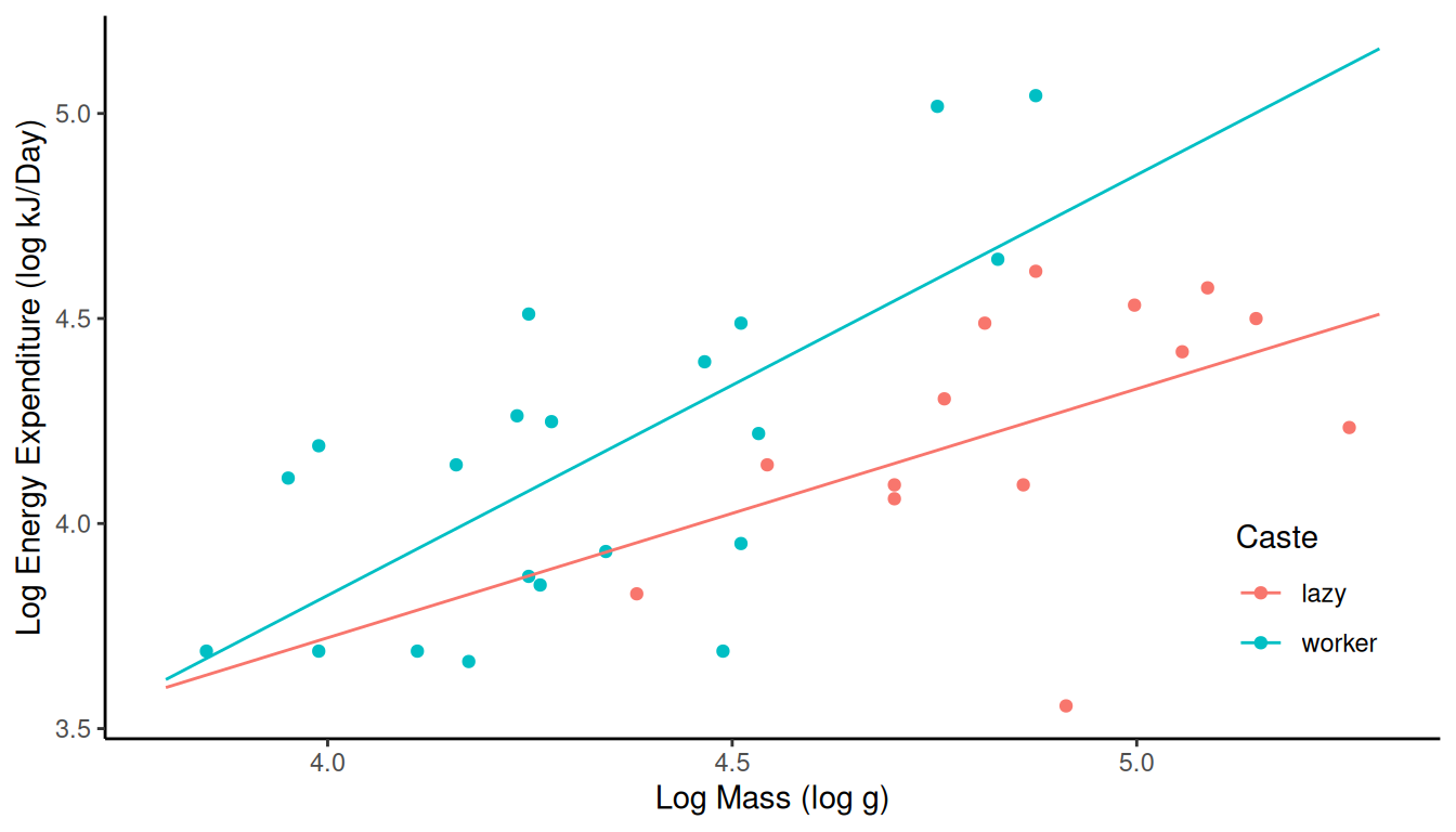

Notice how the “interaction” between log mass and caste now changes the results form contrast since the lines are no longer restricted to be parallel.

contrast(m, a = list(caste = "lazy", ln.mass = c(4,4.5,5)), cnames = c(4,4.5,5))

    estimate      se lower upper tvalue df    pvalue
4      3.722 0.30664 3.096 4.347  12.14 31 2.601e-13
4.5    4.025 0.14787 3.723 4.327  27.22 31 3.313e-23
5      4.328 0.09189 4.141 4.516  47.10 31 2.057e-30

contrast(m, a = list(caste = "worker", ln.mass = c(4,4.5,5)), cnames = c(4,4.5,5))

    estimate      se lower upper tvalue df    pvalue
4      3.825 0.09954 3.622 4.028  38.42 31 1.026e-27
4.5    4.337 0.07665 4.181 4.494  56.59 31 7.432e-33
5      4.850 0.17059 4.502 5.198  28.43 31 9.024e-24

contrast(m, 
  a = list(caste = "worker", ln.mass = c(4,4.5,5)),
  b = list(caste = "lazy", ln.mass = c(4,4.5,5)),
  cnames = c(4,4.5,5))

    estimate     se    lower  upper tvalue df  pvalue
4     0.1032 0.3224 -0.55429 0.7608 0.3202 31 0.75095
4.5   0.3125 0.1666 -0.02715 0.6522 1.8765 31 0.07002
5     0.5219 0.1938  0.12667 0.9171 2.6932 31 0.01131

contrast(m, 
  a = list(caste = c("lazy","worker"), ln.mass = 3),
  b = list(caste = c("lazy","worker"), ln.mass = 2),
  cnames = c("lazy","worker"))

       estimate     se    lower upper tvalue df    pvalue
lazy     0.6069 0.3428 -0.09217 1.306  1.771 31 0.0864587
worker   1.0255 0.2335  0.54928 1.502  4.392 31 0.0001216

Note that for these both the response variable and one explanatory variable have been transformed using a log transformation. Suppose that the transformations had not been yet applied. To simulate this I will create two new variables which are the un-transformed variables.

MoleRats$energy <- exp(MoleRats$ln.energy)
MoleRats$mass <- exp(MoleRats$ln.mass)
summary(MoleRats)

    caste       ln.mass       ln.energy        energy           mass    
 lazy  :14   Min.   :3.85   Min.   :3.56   Min.   : 35.0   Min.   : 47  
 worker:21   1st Qu.:4.25   1st Qu.:3.90   1st Qu.: 49.5   1st Qu.: 70  
             Median :4.51   Median :4.19   Median : 66.0   Median : 91  
             Mean   :4.54   Mean   :4.19   Mean   : 71.0   Mean   :100  
             3rd Qu.:4.84   3rd Qu.:4.49   3rd Qu.: 89.0   3rd Qu.:127  
             Max.   :5.26   Max.   :5.04   Max.   :155.0   Max.   :193

Note that $\exp(x)$ is the inverse transformation of the natural logarithm. If this was the case then we can specify the transformations within the model formula itself.

m <- lm(log(energy) ~ caste + log(mass) + caste:log(mass), data = MoleRats)
summary(m)$coefficients

                      Estimate Std. Error t value Pr(>|t|)
(Intercept)             1.2939     1.6691  0.7752  0.44408
casteworker            -1.5713     1.9518 -0.8050  0.42694
log(mass)               0.6069     0.3428  1.7706  0.08646
casteworker:log(mass)   0.4186     0.4147  1.0094  0.32061

Of course we obtain the same results. But when we make our plot we can put the explanatory variable on its original scale.

d <- expand.grid(caste = c("lazy","worker"), mass = seq(47, 193, length = 100))
d$yhat <- predict(m, newdata = d)

p <- ggplot(MoleRats, aes(x = mass, y = log(energy), color = caste)) +
  geom_point() + theme_minimal() + 
  theme(legend.position = "inside", legend.position.inside = c(0.9, 0.2)) +
  geom_line(aes(y = yhat), data = d) +
  labs(x = "Mass (g)", y = "Log Energy Expenditure (log kJ/Day)", color = "Caste")
plot(p)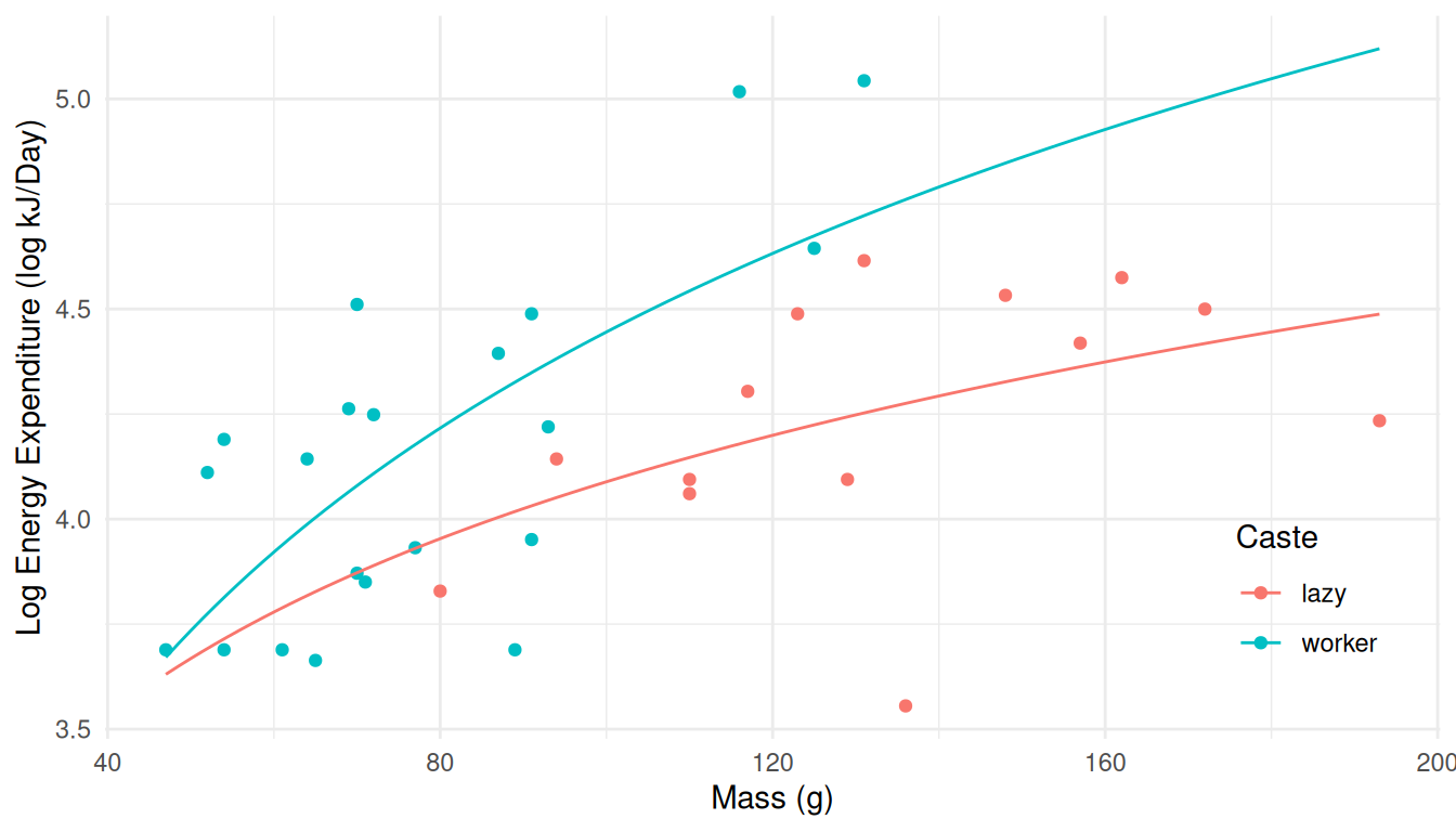

This shows that although this is a linear model, the expected response (the logarithm of the energy expenditure) is not a linear function of mass. And while we could use energy expenditure instead of its logarithm on the ordinate for plotting the data, this does not make sense for the data because we are modeling the expected value of the logarithm of energy expenditure. You cannot “undo” a nonlinear transformation of the response variable because it is not true that $E[f(x)] = f[E(x)]$ where $f(x)$ is some nonlinear function (like log).

Scantlebury, M., Speakman, J. R., Oosthuizen, M. K., Roper, T. J., & Bennett, N. C. (2006). Energetics reveals physiological distinct castes in a eusocial mammal. Nature, 440, 795-797.↩︎