Monday, Nov 11

You can also download a PDF copy of this lecture.

Line-Intercept Sampling

A sample of elements in a region are selected according to the following procedure.

Select a random point within the region based on a uniform distribution. Extend a transect line from that point in a given direction such that it crosses the whole region.
Select all objects that are intercepted by the transect line.

This process can be repeated.

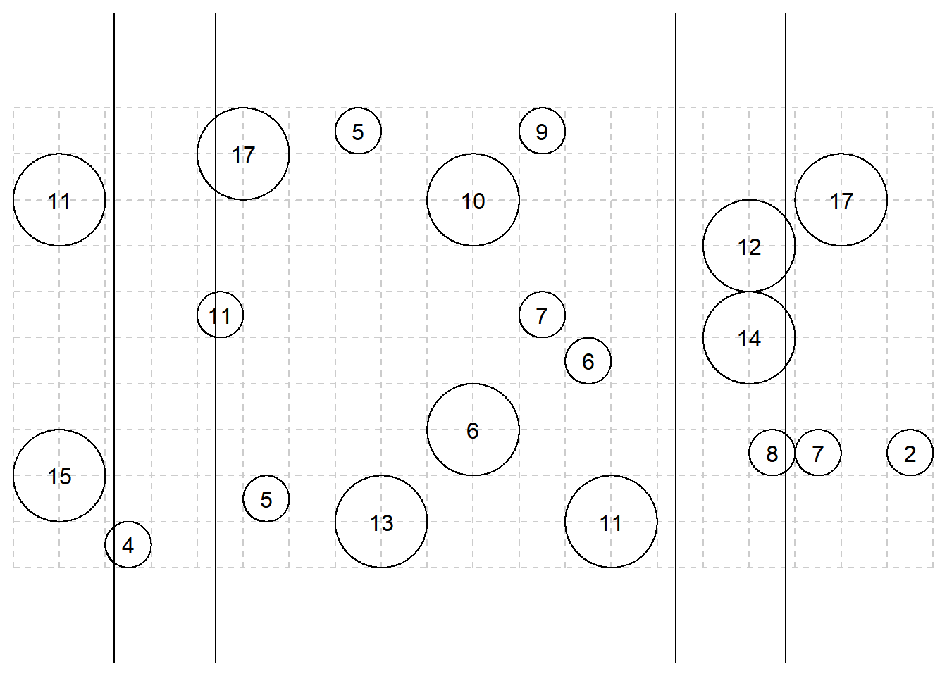
Example: Consider the line-intercept survey with four transect lines.

Consider the sample of objects intercept by one line. The inclusion probability of the $i$-th object is $\pi_i = w_i/W$, where $w_i$ is the horizontal width of the object and $W$ is the total width of the region. An estimator of $\tau$ based on a given line is the Horvitz-Thompson estimator \[ \hat\tau = \sum_{i \in \mathcal{S}} \frac{y_i}{\pi_i} = W\sum_{i \in \mathcal{S}} \frac{y_i}{w_i}. \] Example: Based on the example shown above, what are the estimates of $\tau$ based on the three lines that intercept objects? The value of the target variable is shown within each object.

Let $\hat\tau_k$ be the estimate of $\tau$ based on the $k$-th non-empty line. An estimate of $\tau$ can be obtained by averaging $K$ transect line estimates to get \[ \hat\tau = \frac{1}{K}\sum_{k=1}^K \hat\tau_k. \] The estimated variance of $\hat\tau$ is then \[ \hat{V}(\hat\tau) = \frac{1}{K(K-1)}\sum_{k=1}^K(\hat\tau_k - \hat\tau)^2. \]

Example: What is the estimate of $\tau$ based on the survey given earlier?

Another estimator is to use a Horvitz-Thompson estimator based on the sample of elements intersected by the $n$ transect lines. Then the Horvitz-Thompson estimator is \[ \hat\tau = \sum_{i \in \mathcal{S}}\frac{y_i}{\pi_i}, \] where $\pi_i = 1 - (1 - w_i/W)^t$, since we are sampling with replacement and $w_i/W$ is the selection probability of the $i$-th element. Calculation of the estimated variance of this estimator requires the second-order (joint) inclusion probabilities, which can be computed as \[ \pi_{ij} = \pi_i + \pi_j - 1 + \left(1 - \frac{w_i + w_j - w_{ij}}{W}\right)^t, \] where $w_{ij}/W$ is the probability that objects $i$ and $j$ would both be intersected by a line.

Fixed Area Plot Sampling

A sample of objects in a region are selected according to the following procedure.

Select a random point within the region based on a uniform distribution.
Select all objects that are within a plot of a given shape (e.g., circle, square, or rectangle) centered on that point.

This process can be repeated.

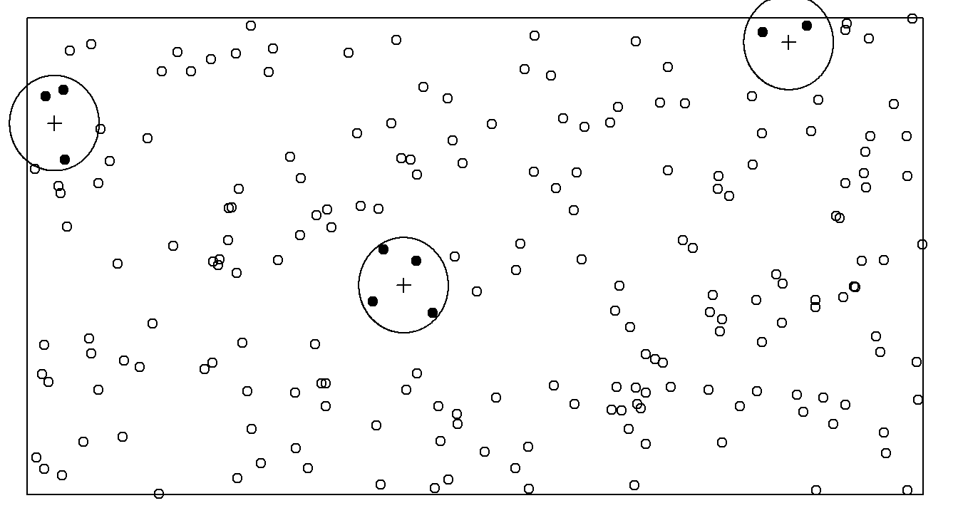
Example: Consider the following fixed area plot survey with three circular fixed area plots.

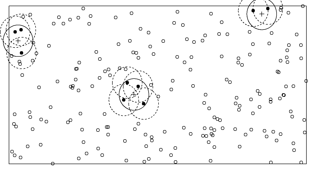
The probability that an object will be included within a plot equals the area of the plot that is also within the region when the center of the plot is centered on the object.

For a given plot the Horvitz-Thompson estimator of $\tau$ is \[ \sum_{i \in \mathcal{S}}\frac{y_{i}}{\pi_{i}} = A\sum_{i \in \mathcal{S}}\frac{y_{i}}{a_{i}}, \] because $\pi_i = a_i/A$ where $A$ is the total area of the region and $a_i$ is the area of the plot that is also withiin the region when the plot is centered on the $i$-th object.

An estimator of $\tau$ can be obtained by averaging these estimates. Let $\hat\tau_k$ be the estimate from the $k$-th non-empty plot. If there are $K$ non-empty plots then the estimator of $\tau$ is \[ \hat\tau = \frac{1}{K}\sum_{k=1}^K \hat\tau_k. \] The estimated variance of $\hat\tau$ is \[ \hat{V}(\hat\tau) = \frac{1}{K(K-1)}\sum_{k=1}^K (\hat\tau_k - \hat\tau)^2. \]

Example: Assume a region with a total area of 5000 meters and $K$ = 3 non-empty circular plots.

$k$	$y_i$	$a_i$
1	63.9	59.5
1	50.4	74.3
1	61.8	75.7
2	27.1	78.5
2	42.0	78.5
2	52.5	78.5
2	33.4	78.5
3	27.8	53.2
3	57.8	47.7

Bitterlich Sampling

A sample of trees is selected according to the following procedure.

Select a random point within a region based on a uniform distribution.
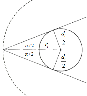
Select all trees with trunk diameters that exceed a critical angle ($\alpha$) when viewed from that point.

Also see Figure 2 in this paper.

Let $\alpha$ be the critical angle and $d_i$ by the diameter of the $i$-th tree. Then the radius ($r_i$) of a circle that encloses all points that would result in the selection of the $i$-th tree is \[ r_i = \frac{d_i}{2\sin(\alpha/2)}. \] Thus the $i$-th tree is selected if and only if \[ \text{distance to center of the $i$-th tree} \le \frac{d_i}{2\sin(\alpha/2)}, \] assuming that this circle does not extend outside the region. The inclusion probability of the $i$-th tree is the probability of this happening. The area of this circle is $a_i = \pi r_i^2$ which can be computed as \[ a_i = \frac{\pi d_i^2}{4\sin^2(\alpha/2)}. \] Note that $\pi$ here is the mathematical constant $\pi$ $\approx$ 3.14, not the inclusion probability of the tree. The inclusion probability of the $i$-th tree is \[ \pi_i = a_i/A, \] where $A$ is the total area of the region in which the point was sampled. If there are $n$ selected trees, then the estimate of $\tau$ for some target variable $y_i$ is \[ \hat\tau = \sum_{i \in \mathcal{S}}\frac{y_i}{\pi_i}. \]

Variations on Bitterlich Sampling

If $y_i$ is the basal area of the $i$-th tree so that $y_i = \pi d_i^2/4$, then \[ \hat\tau = \sum_{i \in \mathcal{S}} \frac{y_i}{\pi_i} = nA \sin^2(\alpha/2), \] where $n$ is the number of selected trees, so that the estimated total basal area is proportional to the number of selected trees.
As in the previous examples if we have $K$ estimates of $\tau$ (based on as many points) then these can be averaged to come up with one estimate. In the case of estimating total basal area, this estimator becomes \[ \hat\tau = \frac{A\sin^2(\alpha/2)}{K}\sum_{k=1}^K n_k, \] so that $\hat\tau$ is proportional to the average number of trees selected.