Friday, Oct 25
You can also download a PDF copy of this lecture.
Optimum Sample Sizes for Two-Stage Cluster Sampling
One of the advantages of two-stage cluster sampling over one-stage cluster sampling is that we have more control over the cost and precision (in terms of the variance of an estimator) of the survey. This is because there are two stages of sampling, and thus two sample size decisions.
- The number of clusters to sample (\(n\)).
- The number of elements to sample from each cluster (\(m_1, m_2, \dots, m_n\)).
Between-Group and Within-Group Mean Squares
Assume a simple case where we have the following.
- Simple random sampling at both stages.
- All clusters are the same size (i.e., all \(M_i\) are equal).
- The number of elements sampled from each cluster are the same (i.e., all \(m_i\) are equal).
To simplify notation, let \(\bar{M} = M/N\) be the number of elements per cluster, and let \(m\) denote the number of elements sampled from each cluster. In this case the unbiased and ratio estimators are the same. Without loss of generality we will consider \(\hat\mu\).
The variance of \(\hat\mu\) can be written as \[ V(\hat\mu) = \left(1 - \frac{n}{N}\right)\frac{\sigma_b^2}{n\bar{M}} + \left(1 - \frac{m}{\bar{M}}\right)\frac{\sigma^2_w}{nm}, \] where \(\sigma_b^2\) and \(\sigma_w^2\) are the mean squares between-groups and within-groups, respectively, defined as \[ \sigma_b^2 = \bar{M}\frac{\sum_{i=1}^N(\mu_i - \mu)^2}{N-1}, \ \ \ \sigma_w^2 = \frac{1}{N}\sum_{i=1}^N \sigma_i^2, \] where \(\mu_i\) and \(\sigma_i^2\) are the mean and variances of the target variable for all the elements in the \(i\)-th cluster.
Example: Consider populations with \(M\) = 1250 elements in \(N\) = 25 clusters, each of size \(\bar{M}\) = 50.
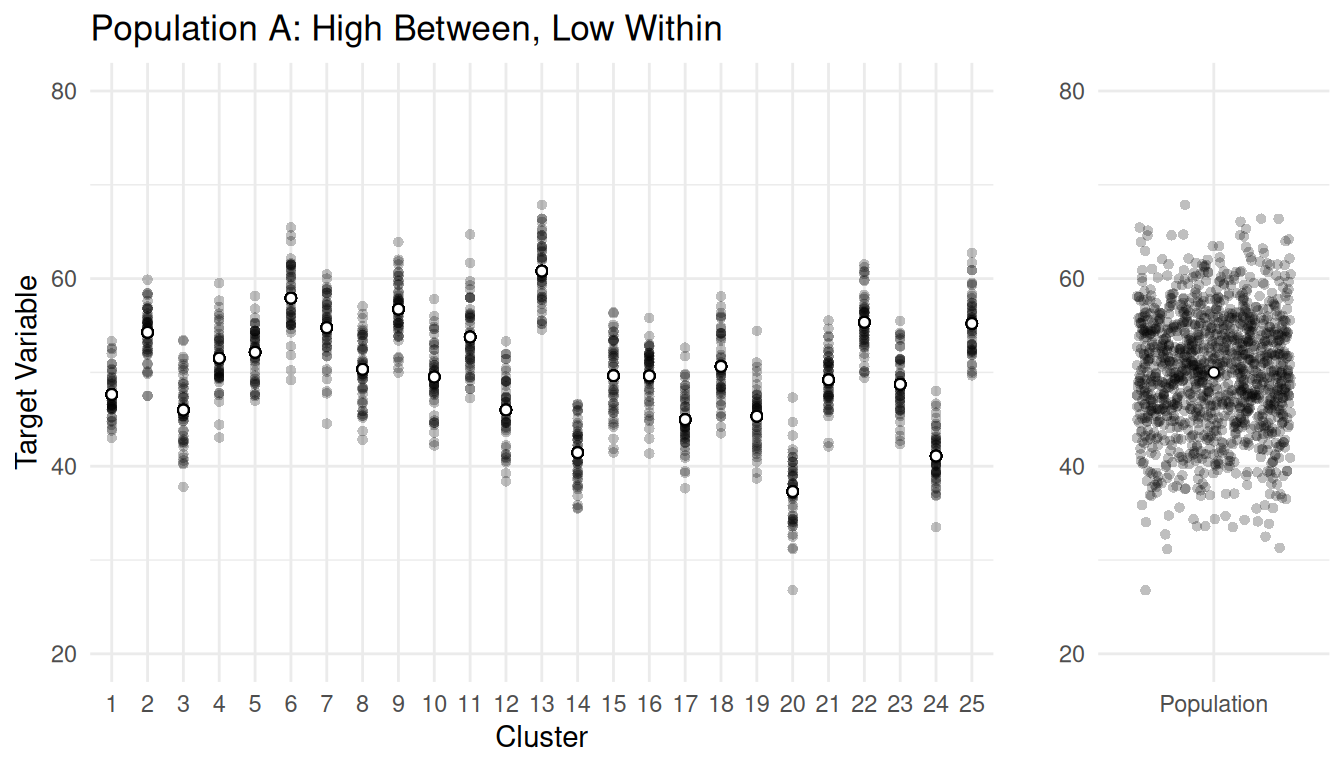
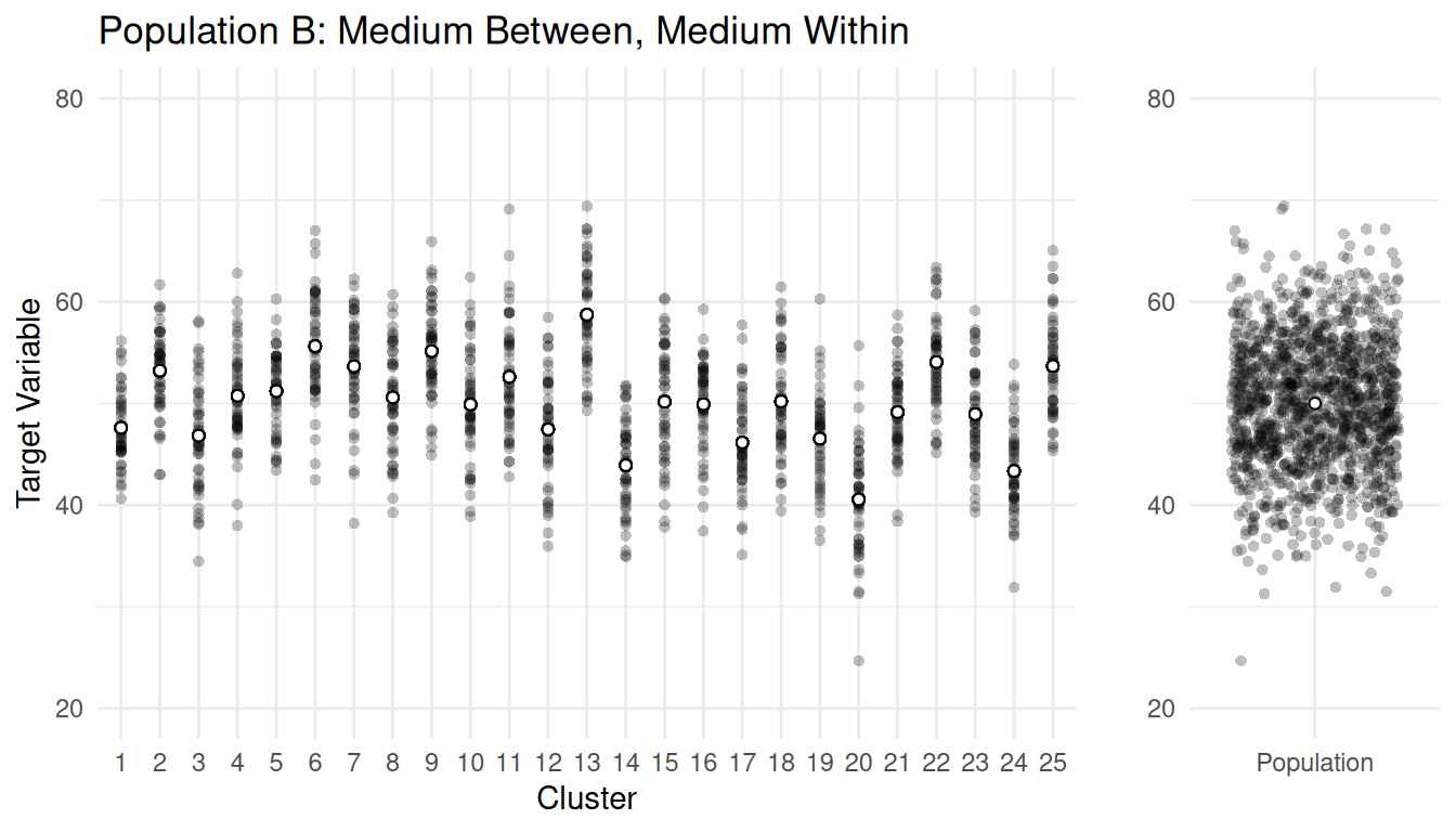
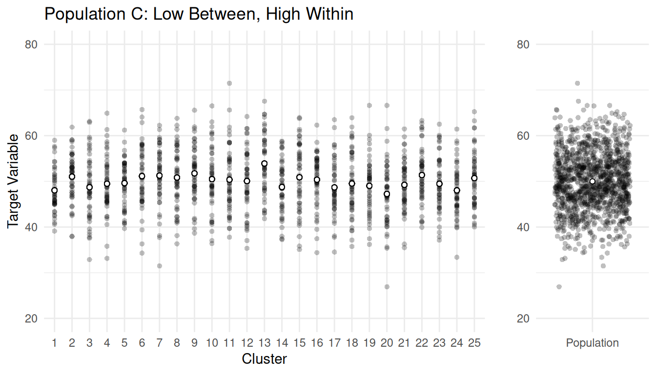
| Population | \(\sigma_b^2\) | \(\sigma_w^2\) |
|---|---|---|
| A | 1551.41 | 10.39 |
| B | 873.23 | 23.68 |
| C | 103.07 | 38.76 |
Optimal Sample Sizes
Assume that the total cost of the survey can be computed as \[ C = nc_1 + nmc_2, \] where \(c_1\) is the cost-per-cluster and \(c_2\) is the cost-per-element. Minimizing cost for a fixed variance or bound, or minimizing the variance or bound for a fixed cost yields \[ m_{\text{opt}} = \sqrt{\frac{\bar{M}\sigma_w^2}{\sigma_b^2 - \sigma_w^2} \times \frac{c_1}{c_2}}. \] Note: We must have \(1 \le m \le \bar{M}\), and \(m_{\text{opt}}\) will not necessarily respect this constraint. Also \(m_{\text{opt}}\) isn’t defined if \(\sigma_b^2 < \sigma_w^2\).
The sample size for the number of clusters (\(n\)) to minimize the variance for a fixed cost is \[ n_{\text{opt}} = \frac{C}{c_1 + c_2m_{\text{opt}}}. \] Note: Clearly we must have \(1 \le n \le N\).
We can encounter various “limiting cases” when solving for \(m_{\text{opt}}\) and \(n_{\text{opt}}\).
- If \(m_{\text{opt}} < 1\) then set \(m_{\text{opt}} = 1\) (i.e., sample just one element per cluster).
- If \(m_{\text{opt}} > \bar{M}\), then set \(m_{\text{opt}} = \bar{M}\) (i.e., use one-stage cluster sampling).
- If \(\sigma_b^2 < \sigma_w^2\) then set \(m_{\text{opt}} = \bar{M}\) (i.e., use one-stage cluster sampling).
- If \(n_{\text{opt}} \ge N\) then set \(n_{\text{opt}} = N\) (i.e., use stratified random sampling).
| Population | \(\sigma_b^2\) | \(\sigma_w^2\) | \(m_{\text{opt}}\) | \(n_{\text{opt}}\) |
|---|---|---|---|---|
| A | 1551.41 | 10.39 | 1.836067 | 8.448752 |
| B | 873.23 | 23.68 | 3.733201 | 7.281624 |
| C | 103.07 | 38.76 | 17.359517 | 3.655035 |
Notice what happens as \(m_{\text{opt}}\) and \(n_{\text{opt}}\) as \(\sigma_b^2\) increases, and notice what happens to \(m_{\text{opt}}\) and \(n_{\text{opt}}\) as \(\sigma_w^2\) increases.
Clearly the solution is approximate — we would need to round the sample sizes.
How do we get \(\sigma_b^2\) and \(\sigma_w^2\) in practice?
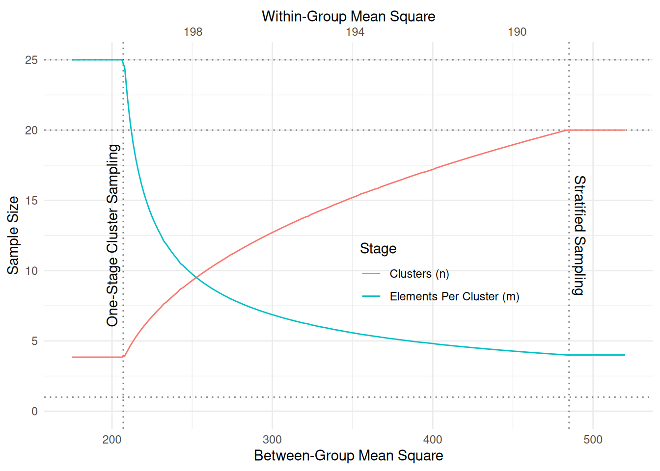
Example: The following plot shows \(m_{\text{opt}}\) and \(n_{\text{opt}}\) as a function of the
between-group and within-group mean squares for a population of \(N\) = 100 clusters with \(\bar{M}\) = 25 elements in each cluster.
The costs are \(c_1\) = 10 and \(c_2\) = 1. The fixed total cost is \(C\) = 100.
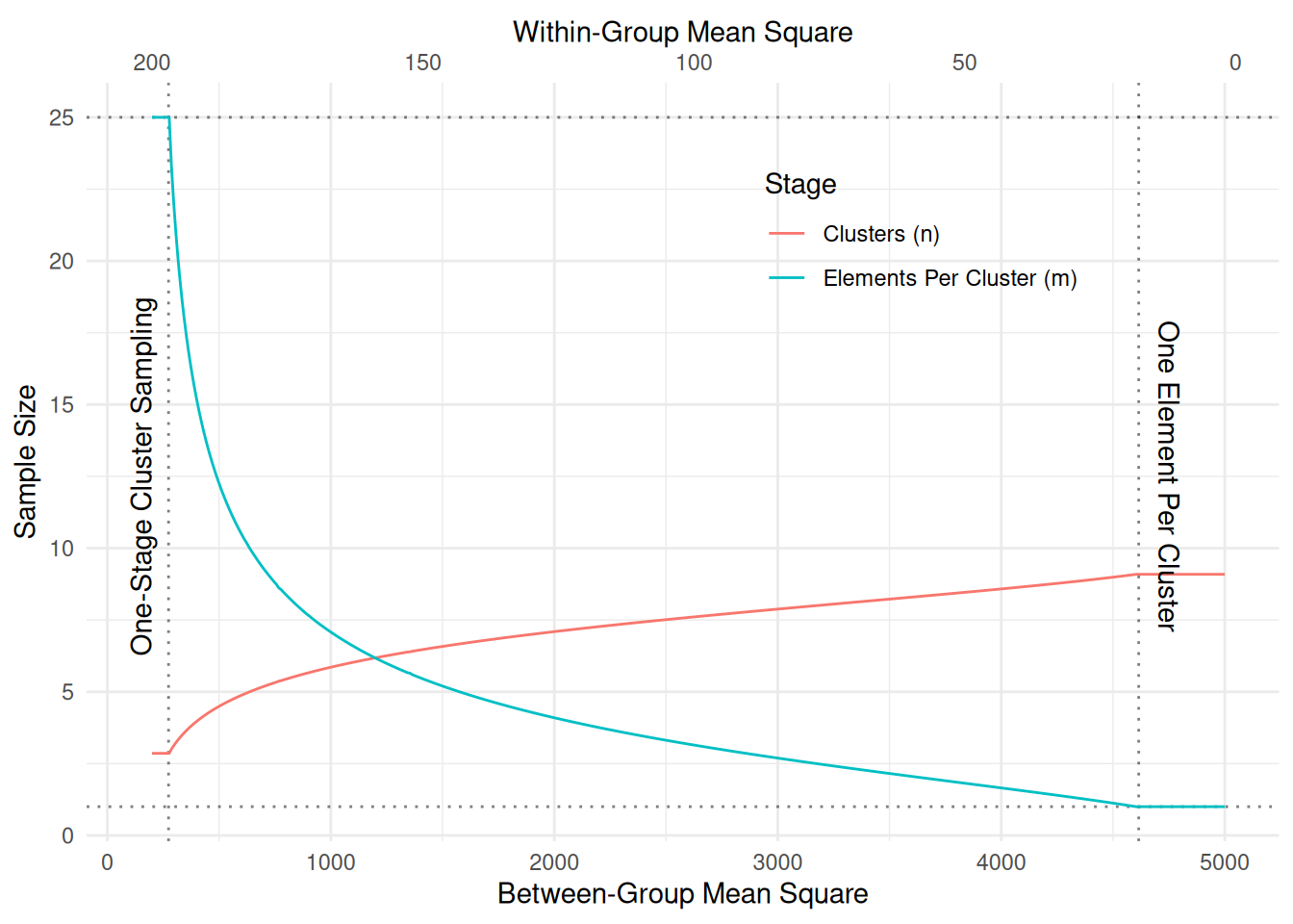
Example: The following plot shows \(m_{\text{opt}}\) and \(n_{\text{opt}}\) as a function of the between-group and within-group mean squares for a population of now \(N\) = 20 clusters, with the cost-per-cluster reduced to \(c_1\) = 1.
Numerical Solution
We can also solve this problem numerically. Here is the numerical solution to the first example above.
library(Rsolnp)

# Function to compute the variance of the estimator.
vf <- function(x, msb, msw, N, Mbar, c1, c2) {
  m <- x[1]
  n <- x[2]
  return((1 - n/N) * msb / (n * Mbar) + (1 - m/Mbar) * msw/(n*m))
}

# Function to compute the cost of the survey.
cf <- function(x, msb, msw, N, Mbar, c1, c2) {
  m <- x[1]
  n <- x[2]
  return(n*c1 + n*m*c2)
}

# Find n and m to minimize the variance subject to the
# constraint that the cost must equal 100.
tmp <- solnp(pars = c(5,5), fun = vf, eqfun = cf, eqB = 100,
  N = 25, Mbar = 50, msb = 1551.41, msw = 10.39, c1 = 10, c2 = 1, LB = c(1,1), UB = c(50,25))
Iter: 1 fn: 3.4968   Pars:  3.71283 7.09572
Iter: 2 fn: 3.1969   Pars:  2.72390 7.80416
Iter: 3 fn: 3.1021   Pars:  2.17386 8.19659
Iter: 4 fn: 3.0797   Pars:  1.90797 8.39335
Iter: 5 fn: 3.0767   Pars:  1.84024 8.44547
Iter: 6 fn: 3.0766   Pars:  1.83610 8.44873
Iter: 7 fn: 3.0766   Pars:  1.83607 8.44875
Iter: 8 fn: 3.0766   Pars:  1.83607 8.44875
solnp--> Completed in 8 iterationstmp$pars[1] 1.836067 8.448752round(tmp$pars)[1] 2 8Multi-Stage Cluster Sampling
A multi-stage cluster sampling design is a natural extension of a two-stage cluster sampling design. A \(k\)-stage cluster sampling design where \(k\) \(\ge\) 2 can be designed by applying clusters sampling designs recursively.
A three-stage cluster sampling design can be described as follows.
- Partition the \(M\) elements in a population into clusters.
- Select \(n_1\) primary sampling units using a probability sampling design.
- For each of the \(n_1\) sampled primary units, partition the elements into sub-clusters.
- Select \(n_2\) secondary sampling units using a probability sampling design.
- For each of the \(n_2\) sampled secondary units, sample tertiary sampling units (i.e., elements) using a probability sampling design, and observe the target variable for these sampled elements.
Multi-stage cluster sampling designs are useful when elements are formed into groups hierarchically. Here are some examples of the three levels of sampling units in three-stage cluster sampling designs.
| primary | secondary | tertiary | Target Variable |
|---|---|---|---|
| pallet | box | widget | weight |
| neighborhood | block | household | income |
| county | farm | field | acres of wheat |
| school | classroom | student | test score |
| day | hour | minute | number of fish |
| plot | sub-plot | tree | volume |
In principle, any probability sampling design can be used at each stage. But often only the first stage uses a design other than SRS (e.g., PPS, stratified random sampling). Tyipcally later stages use SRS.