Inclusion Probabilities in Design and Estimation
You can also download a PDF copy of this document.
Computing Inclusion Probabilities
Suppose we have the following sampling design for a population of five elements. \[\begin{align*} \mathcal{S}_1 & = \{\mathcal{E}_1,\mathcal{E}_3,\mathcal{E}_4\}, \ P(\mathcal{S}_1) = 0.1 \\ \mathcal{S}_2 & = \{\mathcal{E}_1,\mathcal{E}_3,\mathcal{E}_5\}, \ P(\mathcal{S}_2) = 0.1 \\ \mathcal{S}_3 & = \{\mathcal{E}_1,\mathcal{E}_4,\mathcal{E}_5\}, \ P(\mathcal{S}_3) = 0.1 \\ \mathcal{S}_4 & = \{\mathcal{E}_2,\mathcal{E}_3,\mathcal{E}_4\}, \ P(\mathcal{S}_4) = 0.2 \\ \mathcal{S}_5 & = \{\mathcal{E}_2,\mathcal{E}_3,\mathcal{E}_5\}, \ P(\mathcal{S}_5) = 0.2 \\ \mathcal{S}_6 & = \{\mathcal{E}_2,\mathcal{E}_4,\mathcal{E}_5\}, \ P(\mathcal{S}_6) = 0.3 \\ \end{align*}\] The table below shows the first-order (\(\pi_i\)) and second-order (\(\pi_{ij}\)) inclusion probabilities for the five elements in the population.| i | 1 | 2 | 3 | 4 | 5 |
|---|---|---|---|---|---|
| 1 | 0.3 | 0.0 | 0.2 | 0.2 | 0.2 |
| 2 | 0.0 | 0.7 | 0.4 | 0.5 | 0.5 |
| 3 | 0.2 | 0.4 | 0.6 | 0.3 | 0.3 |
| 4 | 0.2 | 0.5 | 0.3 | 0.7 | 0.4 |
| 5 | 0.2 | 0.5 | 0.3 | 0.4 | 0.7 |
Note that the values along the “diagonal” (i.e., from top left to bottom right) are the first-order inclusion probabilities, whereas the values not along this diagonal are the second-order inclusion probabilities. The reason why it makes sense to represent the inclusion probabilities this way is that the second-order inclusion probability of an element with itself (e.g., \(\pi_{ii}\)) equals the first-order inclusion probability (e.g., \(\pi_i\)). Verify these inclusion probabilities by computing them yourself from the sampling design. Note that the second-order inclusion probabilities are symmetric in the sense that \(\pi_{ij} = \pi_{ji}\) so you only need to verify five first-order inclusion probabilities and ten second-order inclusion probabilities.
Computing the Horvitz-Thompson Estimator
Consider the sampling design given in the previous problem. Assume that \(y_1\) = 1, \(y_2\) = 2, \(y_3\) = 4, \(y_4\) = 2, and \(y_5\) = 1. Confirm that the estimates of \(\tau\) using the Horvitz-Thompson estimator are, approximately, 12.86, 11.43, 7.62, 12.38, 10.95, and 7.14 for samples \(\mathcal{S}_1\), \(\mathcal{S}_2\), \(\mathcal{S}_3\), \(\mathcal{S}_4\), \(\mathcal{S}_5\), and \(\mathcal{S}_6\), respectively. Also use the Horvitz-Thompson estimator to compute an estimate of \(\mu\) two ways: one assuming you know that the number of elements in the population is known to be five, and another where the number of elements in the population is unknown. You should confirm that the estimates based on the six samples with a known number of elements in the population are approximately 2.57, 2.29, 1.52, 2.48, 2.19, and 1.43, respectively, and that the estimates based on the six samples with an unknown number of elements in the population are approximately 2, 1.78, 1.23, 2.74, 2.42, and 1.67, respectively.
Generalized Horvitz-Thompson Estimator
Consider the sampling design described in the previous problems. Suppose that we have an auxiliary variable \(x_i\) where \(x_1\) = 9, \(x_2\) = 21, \(x_3\) = 18, \(x_4\) = 21, and \(x_5\) = 21, and it is known that \(\tau_x\) = 90. Verify that the generalized Horvitz-Thompson estimator that is based on the ratio estimator produces an estimate of \(\hat\tau_y\) \(\approx\) 12.9 if the sample is \(\mathcal{S}_1\).
Sampling With Replacement
Consider the population of four elements, \(\mathcal{P} = \{\mathcal{E}_1,\mathcal{E}_2,\mathcal{E}_3,\mathcal{E}_4\}\). Assume that the sample \(\mathcal{S} = \{\mathcal{E}_1,\mathcal{E}_1,\mathcal{E}_4\}\) selected using sampling with replacement with given selection probabilities. The table below shows the value of the target variable for each element in the population and its selection probability.| Element | \(y_i\) | \(\delta_i\) |
|---|---|---|
| \(\mathcal{E}_1\) | 4 | 0.1 |
| \(\mathcal{E}_2\) | 1 | 0.2 |
| \(\mathcal{E}_3\) | 2 | 0.3 |
| \(\mathcal{E}_4\) | 3 | 0.4 |
Confirm that the estimate of \(\tau\) using the Hansen-Hurwitz estimator approximately 29.17, and that the estimate of \(\tau\) using the Horvitz-Thompson estimator is approximately 18.59.
Line-Intercept Sampling
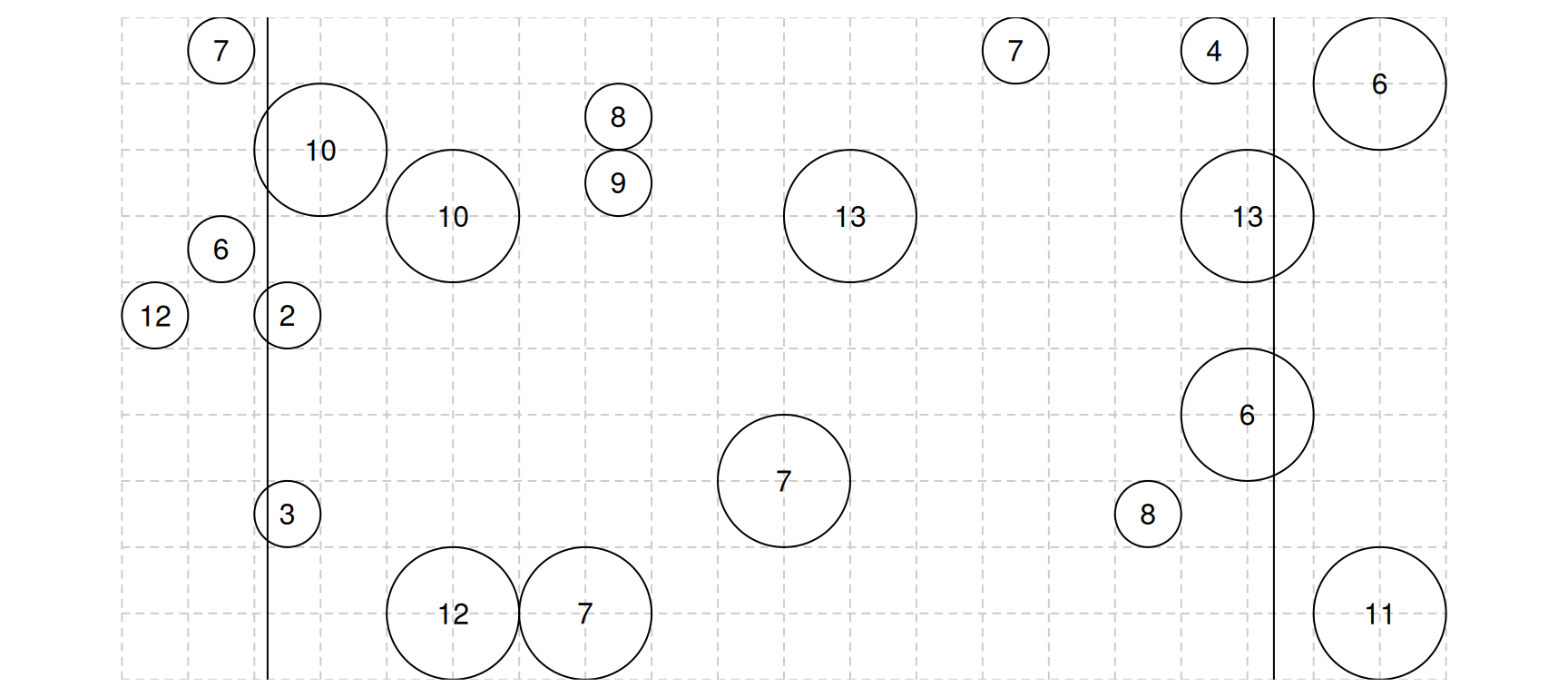
The figure below shows the the results of a survey using the
line-intercept method. The selected objects, represented by circles, are
those intercepted by the two transect lines. The value of the target
variable is shown as the number within each object.
 Confirm that the estimates of \(\tau\)
based on the left and right transect lines are 200 and 190,
respectively, using the Horvitz-Thompson estimator. These can be
averaged together to produce and estimate of \(\tau\) of 195.
Using Survey Weights
Suppose you have only the following information about a survey with an unknown design: the values of the target variable and the corresponding survey weights for the three elements in the sample.| Target Variable | Survey Weight |
|---|---|
| 5 | 4.0 |
| 3 | 2.5 |
| 2 | 2.0 |
Verify that based on this information alone an estimate of \(\tau\) is \(\hat\tau\) \(=\) 31.5, and an estimate of \(\mu\) is \(\hat\mu\) \(\approx\) 3.7.