Monday, Apr 3
You can also download a PDF copy of this lecture.
Independent Versus Dependent Samples
Example: Consider a study like the twin study for investigating the relationship between schizophrenia and the volume of the left hippocampus.| Pair | Unaffected | Affected | Difference |
|---|---|---|---|
| 1 | 1.94 | 1.27 | 0.67 |
| 2 | 1.44 | 1.63 | -0.19 |
| 3 | 1.56 | 1.47 | 0.09 |
| 4 | 1.58 | 1.39 | 0.19 |
| 5 | 2.06 | 1.93 | 0.13 |
| 6 | 1.66 | 1.26 | 0.4 |
| 7 | 1.75 | 1.71 | 0.04 |
| 8 | 1.77 | 1.67 | 0.1 |
| 9 | 1.78 | 1.28 | 0.5 |
| 10 | 1.92 | 1.85 | 0.07 |
| 11 | 1.25 | 1.02 | 0.23 |
| 12 | 1.93 | 1.34 | 0.59 |
| 13 | 2.04 | 2.02 | 0.02 |
| 14 | 1.62 | 1.59 | 0.03 |
| 15 | 2.08 | 1.97 | 0.11 |
| Size: | 15 | 15 | 15 |
| Mean: | 1.759 | 1.56 | 0.199 |
| SD: | 0.242 | 0.301 | 0.238 |
How would we make inferences if the samples are dependent, and how would we make inferences if the samples are independent?
Matching in Observational Studies
Example: Consider a study to compare the foot hair density of Hobbits who smoke pipe-weed with that of Hobbits that do not smoke. But we use an observational study and are concerned that smoking and foot hair density are also related to the confounding variables age and Farthing. We can control for age and Farthing by matching Hobbits based on those two variables.| Pair | Age | Farthing | FHDI | FHDI | Farthing | Age | |
|---|---|---|---|---|---|---|---|
| 1 | 60 | W | 74.8 | 70.1 | W | 59 | |
| 2 | 108 | W | 96.2 | 45.1 | W | 109 | |
| 3 | 80 | E | 69.3 | 60.2 | E | 80 | |
| 4 | 43 | N | 96.9 | 76.3 | N | 43 | |
| 5 | 96 | S | 77.6 | 69.2 | S | 96 | |
| \(\vdots\) | \(\vdots\) | \(\vdots\) | \(\vdots\) | \(\vdots\) | \(\vdots\) | \(\vdots\) | |
| 100 | 98 | W | 70.5 | 49 | W | 95 |
| Pair | Smoker | Non-Smoker | Difference |
|---|---|---|---|
| 1 | 74.8 | 70.1 | 4.7 |
| 2 | 96.2 | 45.1 | 51.1 |
| 3 | 69.3 | 60.2 | 9.1 |
| 4 | 96.9 | 76.3 | 20.6 |
| 5 | 77.6 | 69.2 | 8.4 |
| \(\vdots\) | \(\vdots\) | \(\vdots\) | \(\vdots\) |
| 100 | 70.5 | 49 | 21.5 |
Standard Errors for Dependent Versus Independent Samples
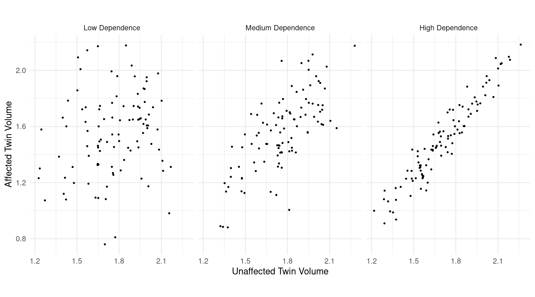
Suppose we have two samples, both of equal size \(n\) (so we’ll leave off the subscript). The standard error of \(\bar{x}_1-\bar{x}_2\) is \[ \underbrace{\sqrt{\frac{\sigma_1^2}{n} + \frac{\sigma_2^2}{n}}}_{\text{independent}} \ge \underbrace{\sqrt{\frac{\sigma_1^2}{n} + \frac{\sigma_2^2}{n} - \rho\frac{2\sigma_1\sigma_2}{n}}}_{\text{dependent}} = \frac{\sigma_d}{\sqrt{n}}. \] Here \(\sigma_d\) is the standard deviation of the differences of matched observations, and \(\rho\) is the correlation coefficient. The correlation coefficient can be between -1 and 1.
- If the samples are independent then \(\rho = 0\).
- If the samples are dependent then (usually) \(0 < \rho < 1\).
What does this imply about the standard errors for dependent versus independent samples?
Example: Suppose we had a matched-pairs design using
genetically-related individuals (e.g., cousins, siblings, or identical
twins) for a study like that that investigated the relationship between
schizophrenia and left hippocampus volume.

The Other Standard Error for \(\bar{x}_1-\bar{x}_2\)
If two samples are independent, the standard error we have been using is \[ \sqrt{\frac{s_1^2}{n_1} + \frac{s_2^2}{n_2}}. \] An alternative is to use \[ s\sqrt{\frac{1}{n_1} + \frac{1}{n_2}}, \ \ \ \text{where} \ \ \ s = \sqrt{\frac{(n_1-1)s_1^2 + (n_2-1)s_2^2}{n_1 + n_2 - 2}}, \] and the degrees of freedom becomes \(n_1 + n_2 - 2\).
Why would we use this alternative standard error?