Wednesday, Jan 11

The “Anatomy” of (Typical) Data

What do data look like?

Example: The following are fictional data consisting of 20 observations of the Hobbits attending a party at the Prancing Pony Inn in the town of Bree.

Observation	Name	Farthing	Height
1	Arbogastes Goodwort	East	104 cm
2	Britius Thornburrow	East	95 cm
3	Hamfast Fleetfoot	East	96 cm
4	Polo Chubb-Baggins	South	93 cm
5	Berengar Longbottom	East	86 cm
6	Meginhard Galpsi	South	109 cm
7	Fulrad Boffin	South	96 cm
8	Fortinbras Boffin	South	72 cm
9	Sigefroy Roper	East	99 cm
10	Dado Zaragamba	North	87 cm
11	Ingunde Proudfoot	West	81 cm
12	Taryn Zaragamba	South	89 cm
13	Vuldretrada Mugwort	South	81 cm
14	Bailey Hedgehopper	North	84 cm
15	Rose Smallburrow	South	85 cm
16	Merofled North-took	East	75 cm
17	Duenna Undertree	West	100 cm
18	Asphodel Swiftfoot	North	93 cm
19	Daisy Townsend	East	80 cm
20	Madeline Underfoot	East	104 cm

Example: The following are data from a study by Charles Darwin that compared the heights of seedlings produced by cross-fertilization versus self-fertilization.¹ Each observation is the heights (in inches) of a pair of seedlings from two flowers on the same parent plant, as well as the difference in the heights.

	Fertilization
Obs	Cross	Self	Difference
1	23.500	17.375	6.125
2	12.000	20.375	-8.375
3	21.000	20.000	1.000
4	22.000	20.000	2.000
5	19.125	18.375	0.750
6	21.500	18.625	2.875
7	22.125	18.625	3.500
8	20.375	15.250	5.125
9	18.250	16.500	1.750
10	21.625	18.000	3.625
11	23.250	16.250	7.000
12	21.000	18.000	3.000
13	22.125	12.750	9.375
14	23.000	15.500	7.500
15	12.000	18.000	-6.000

The fundamental unit of data is the observation (one row of the table of data shown above). An observation is the set of values of one or more variables.

Variables are characteristics of the observation. One basic distinction is between quantitative (i.e., numerical) and categorical variables (i.e., qualitative).

Samples and Populations

An important issue in statistics is that we often do not observe all possible observations.

A sample is the set of observed observations.

A population is the set of all possible observations — both observed and unobserved. A population can be real and finite (e.g., most surveys), or hypothetical and infinite (e.g., laboratory studies).

Note: Sometimes the sample and population are defined in terms of the objects (e.g., Hobbits, seedling pairs) on which the observations are made. This is particularly true in surveys. But for greater generality we will define samples and populations in terms of observations.

Example: The observations in black below are the observed observations (i.e., the sample). The observations in grey below are the unobserved observations. We might define all 20 observations as the population.

Observation	Name	Farthing	Height
1	Arbogastes Goodwort	East	104 cm
2	Britius Thornburrow	East	95 cm
3	Hamfast Fleetfoot	East	96 cm
4	Polo Chubb-Baggins	South	93 cm
5	Berengar Longbottom	East	86 cm
6	Meginhard Galpsi	South	109 cm
7	Fulrad Boffin	South	96 cm
8	Fortinbras Boffin	South	72 cm
9	Sigefroy Roper	East	99 cm
10	Dado Zaragamba	North	87 cm
11	Ingunde Proudfoot	West	81 cm
12	Taryn Zaragamba	South	89 cm
13	Vuldretrada Mugwort	South	81 cm
14	Bailey Hedgehopper	North	84 cm
15	Rose Smallburrow	South	85 cm
16	Merofled North-took	East	75 cm
17	Duenna Undertree	West	100 cm
18	Asphodel Swiftfoot	North	93 cm
19	Daisy Townsend	East	80 cm
20	Madeline Underfoot	East	104 cm

The population includes \(N\) = 20 observations. The sample (also shown below) contains \(n\) = 5 observations. The symbols \(N\) and \(n\) are called the size of the population and sample, respectively (i.e., the number of observations in the population or sample).

Observation	Name	Farthing	Height
1	Ingunde Proudfoot	West	81 cm
2	Taryn Zaragamba	South	89 cm
3	Bailey Hedgehopper	North	84 cm
4	Merofled North-took	East	75 cm
5	Duenna Undertree	West	100 cm

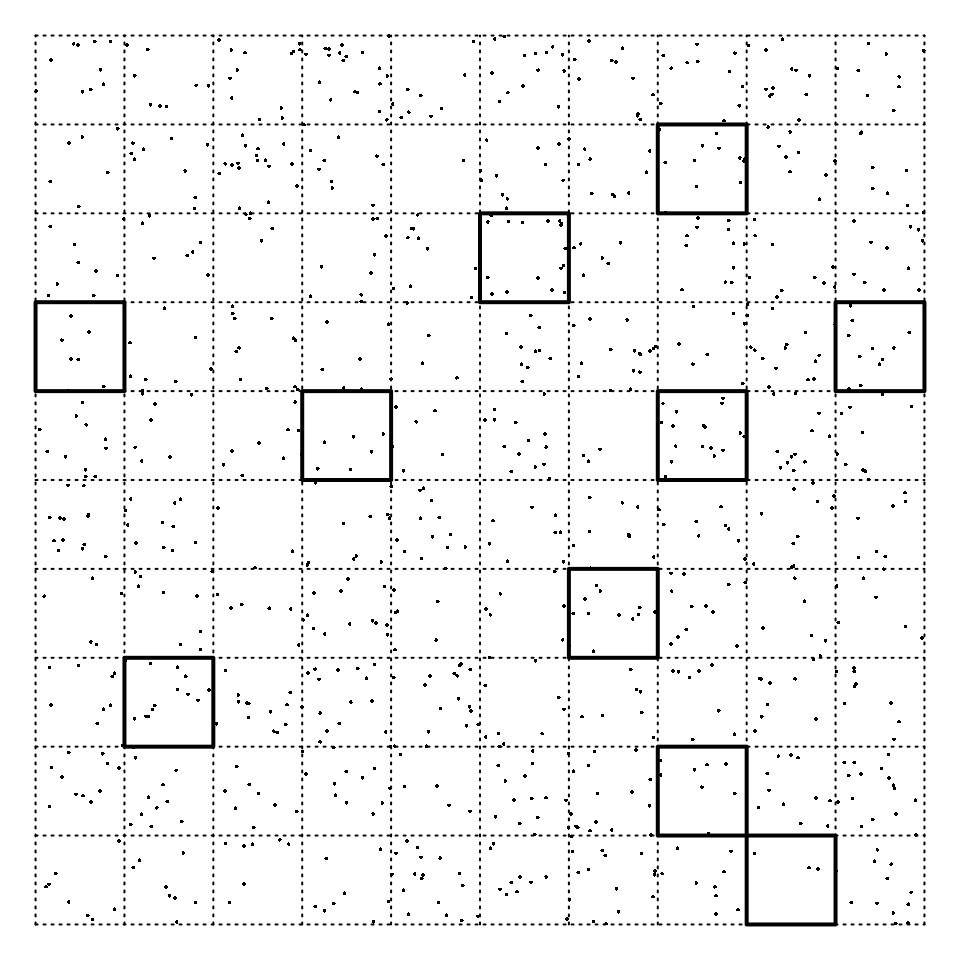
Example: Consider a rectangular-shaped piece of land that has been divided into 100 smaller rectangular units, each containing something of interest (e.g., trees, burrows, archaeological artifacts). A subset of 10 of those smaller units was selected and the number of objects in each of these units was counted. Here we have a population size of \(N\) = 100 and a sample size of \(n\) = 10.

Example: Consider Charles Darwin’s study of the difference in height of corn seedlings produced from cross-fertilization verses self-fertilization. There were two seedlings from each plant — one from a seed produced by cross-fertilization, and another from a seed produced by self-fertilization

	Height
Obs	Cross	Self	Diff
1	23.500	17.375	6.125
2	12.000	20.375	-8.375
3	21.000	20.000	1.000
4	22.000	20.000	2.000
5	19.125	18.375	0.750
6	21.500	18.625	2.875
7	22.125	18.625	3.500
8	20.375	15.250	5.125
9	18.250	16.500	1.750
10	21.625	18.000	3.625
11	23.250	16.250	7.000
12	21.000	18.000	3.000
13	22.125	12.750	9.375
14	23.000	15.500	7.500
15	12.000	18.000	-6.000
16	18.125	18.250	-0.125
17	19.625	18.875	0.750
18	26.250	18.500	7.750
\(\vdots\)	\(\vdots\)	\(\vdots\)	\(\vdots\)

Note that here the sample size is \(n\) = 15, but the population size is effectively infinite (i.e., \(N\) = \(\infty\)).

Statistics and Parameters

A statistic is a description of the observations in a sample.

A parameter is a description of the observations in a population.

Note: More formally, a statistic is anything that is a function of the observations in a sample, and a parameter is a function of the observations in a population.

Descriptive and Inferential Statistics

Descriptive statistics concerns describing the observations in a sample using statistics, or a population using parameters.

Inferential statistics (or statistical inference) concerns using a sample (usually a statistic) to make conclusions about a population (usually a parameter).

The “Big Picture”

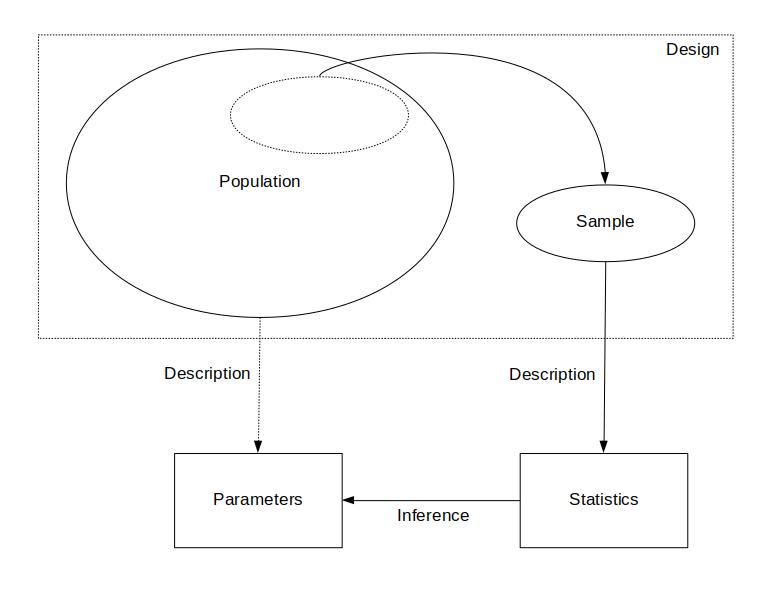
The “big picture” illustrates the roles of population versus sample, design, parameter versus statistic, and description versus inference. The design of a study is the process of how we obtain a sample — i.e., how we collect data (more on that later).