Homework Problem Set 4: Probability Distributions
You can also download a PDF copy of this homework assignment.
Note: The solutions are given within each problem by asking you to confirm the answer.
Means and Standard Deviations of Discrete Random Variables
Consider a survey of tree volume. Suppose that in the population of trees 10% have a volume of 10 cubic feet, 20% have a volume of 20 cubic feet, 30% have a volume of 30 cubic feet, and 40% have a volume of 40 cubic feet. Let \(x\) denote the volume of a randomly selected tree, assuming that every tree has an equal chance of being selected. The probability distribution of \(x\) is given in the table below.
\(x\)
\(P(x)\)
10
0.1
20
0.2
30
0.3
40
0.4
This is what we would call a population distribution since it is the probability distribution of a single observation (and also happens to correspond to the distribution of observations in the population if we think of the probabilities as relative frequencies). Confirm that \(x\) has a mean of \(\mu\) = 30 cubic feet and a standard deviation of \(\sigma\) = 10 cubic feet by computing them yourself.
Now consider the probability distribution of the mean volume (\(\bar{x}\)) of the observed volumes of \(n\) = 2 trees, selected at random based on the distribution given above. Recall that the probability distribution of a statistic, like \(\bar{x}\), is called a sampling distribution. This probability distribution is shown in the table below.
\(\bar{x}\)
\(P(\bar{x})\)
10
0.01
15
0.04
20
0.10
25
0.20
30
0.25
35
0.24
40
0.16
Confirm that the mean, variance, and standard deviation of \(\bar{x}\) are 30, 50, and approximately 7.07, respectively.
Recall the example from class where we observe whether a female platy prefers the yellow-tailed or the clear-tailed male. Let \(x\) denote the preference and assume the following probability distribution.
\(x\)
\(P(x)\)
clear
0.3
yellow
0.7
If we observe a sample of \(n\) = 2 observations and compute the proportion of those observations in which the yellow-tailed male is preferred (which we denote as \(\hat{p}\)), then the sampling distribution of \(\hat{p}\) is as follows.
\(\hat{p}\)
\(P(\hat{p})\)
0.0
0.09
0.5
0.42
1.0
0.49
Confirm that the mean of \(\hat{p}\) is 0.7, and that the standard deviation of \(\hat{p}\) is approximately 0.32.
Computing Probabilities from Discrete Probability Distributions
Consider again the sampling distribution of the mean volume (\(\bar{x}\)) of a sample of \(n\) = 2 trees.
\(\bar{x}\)
\(P(\bar{x})\)
10
0.01
15
0.04
20
0.10
25
0.20
30
0.25
35
0.24
40
0.16
Use this distribution to confirm that the probability that \(\bar{x}\) is less than 20 is 0.05, the probability that \(\bar{x}\) is greater than 30 is 0.4, and that the probability that \(\bar{x}\) is both greater than 15 and less than 35 is 0.55.
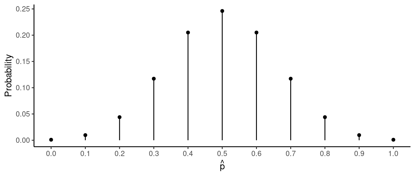
Suppose a fair coin is flipped 10 times and compute the proportion of flips on which the coin comes up heads. We can think of this proportion, \(\hat{p}\), as a statistic for a sample of \(n\) = 10 observations. The sampling distribution of this statistic is shown below using a plot and also a table.

\(\hat{p}\)
\(P(\hat{p})\)
0.0
0.001
0.1
0.010
0.2
0.044
0.3
0.117
0.4
0.205
0.5
0.246
0.6
0.205
0.7
0.117
0.8
0.044
0.9
0.010
1.0
0.001
Use this distribution to confirm that the probability that the proportion of heads is between 0.3 and 0.7 (meaning that it is greater than 0.3 and less than 0.7) is 0.656, the probability that the proportion of heads is between 0.2 and 0.8 (meaning that it is greater than 0.2 and less than 0.8) is 0.89, the probability that the proportion of heads is greater than 0.6 is 0.172, and the probability that the proportion of heads is greater than 0.7 is 0.055.
Computing Probabilities from Continuous Probability Distributions
The figure below shows the probability distribution of a
continuous random variable \(x\).
 Use this figure to confirm the following probabilities by computing them
yourself.
- The probability of \(x < 2\) is 0.2.
- The probability of \(x > 2\) is 0.8.
- The probability of \(2 < x < 4\) is 0.4.
- The probability of \(4 < x < 6\) is 0.3.
- The probability of \(2 < x < 6\) is 0.7.
- The probability of \(3 < x < 5\) is 0.35.
- The probability of \(x > 5\) is 0.25.
- The probability of \(x = 3\) is 0.
- The probability of \(0 < x < 0.5\) is 0.05.
- The probability of \(x > 6.5\) is 0.075.
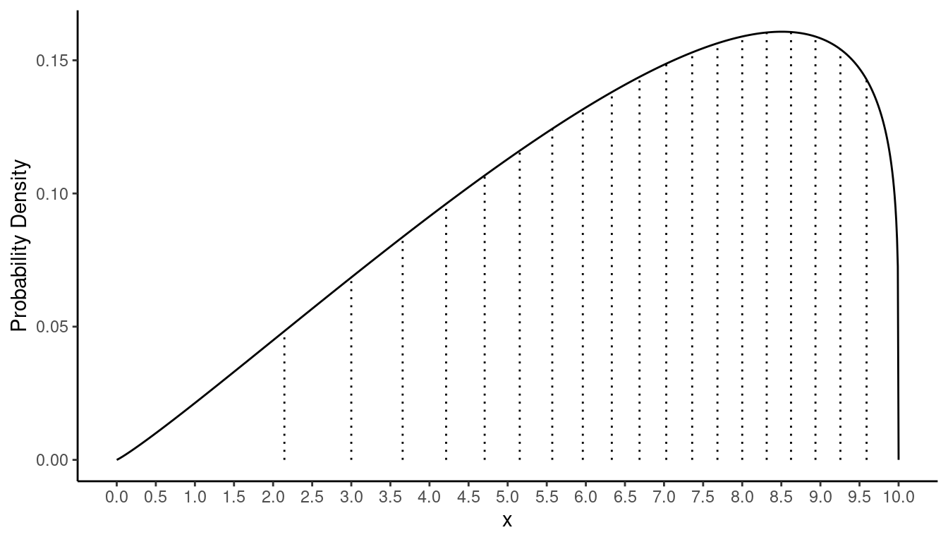
The figure below shows the probability distribution of a continuous
random variable \(x\).
 The vertical dotted line segments divide the total area under the curve
into 20 areas of equal size, so each slice has an area of 1/20 = 0.05.
Use the figure to confirm the following probabilities.
The probability of \(x < 3\) is 0.1.
The probability of \(x < 8\) is 0.7.
The probability of \(x > 3\) is 0.9.
The probability of \(x > 8\) is 0.3.
The probability of \(3 < x < 8\) is 0.6.
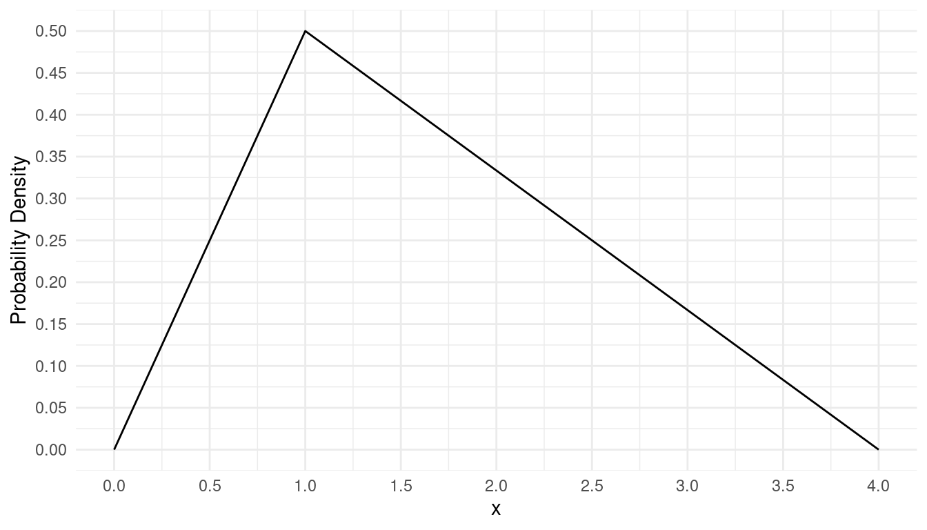
The figure below shows what is sometimes called a triangular
distribution.
 Use this figure to confirm the following probabilities. (Hint: The area
of a right triangle is base times height divided by two.)
The probability of \(x < 1\) is 0.25.
The probability of \(x > 1\) is 0.75.
The probability of \(x < 0.5\) is 0.0625.
The probability of \(x > 2.5\) is 0.1875.
The probability of \(0.5 < x < 2.5\) is 0.75.
Quartiles of the Probability Distribution of a Continuous Random Variable
The figure below shows the probability distribution of a
continuous random variable \(x\).
 Consider the problem of finding the quartiles. By definition, the first
quartile is a number \(Q_1\) such that
the probability of \(x < Q_1\) is
0.25. Similarly we can define the second and third quartiles by the fact
that the probability of \(x < Q_2\)
is 0.5, and that the probability of \(x <
Q_3\) is 0.75 (also the probability of \(x > Q_1\) is 0.75, the probability of
\(x > Q_2\) is 0.5, and the
probability of \(x > Q_3\) is 0.25).
For example, in the first problem in this section \(Q_3 = 5\) because there the probability of
\(x > 5\) is 0.25. Find the
quartiles. (Hint: You will know if you have the correct numbers if the
probabilities described above are correct for those numbers. For
example, you will know if you have found \(Q_1\) if the probability of \(x < Q_1\) is 0.25. Also, all three
quartiles are whole numbers for this distribution.)
Computing Probabilities from the Normal Distribution
Consider a survey of black cherry trees in a forest where the
variable of interest is the heights of the trees (in feet). Let \(x\) denote the height of a single tree is
randomly selected from the forest, and suppose that the probability
distribution of \(x\) (i.e., the
population distribution) is approximately normal in shape with
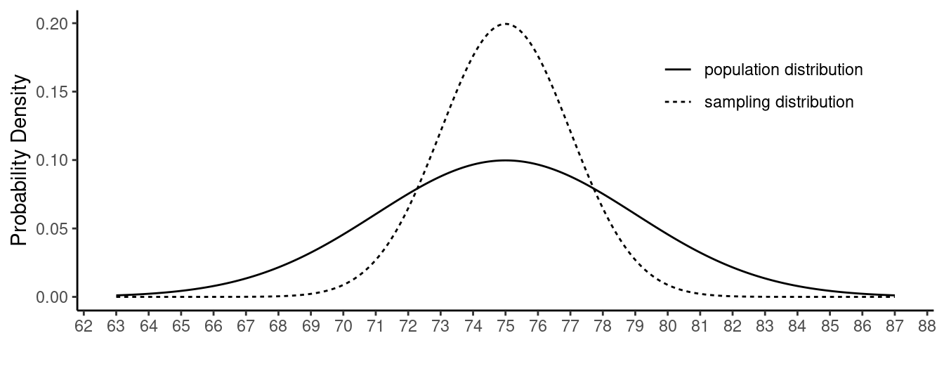
mean 75 and standard deviation 4. Let \(\bar{x}\) denote the mean height of the
trees in a sample of \(n\) = 4 trees
selected at random. The probability distribution of \(\bar{x}\) (i.e., the sampling
distribution) is also approximately normal with a mean of 75 and a
standard deviation of 2. The figure below shows these two distributions.
 Use the population distribution described above to confirm the
following probabilities. You can use statdistributions.com to
compute probabilities based on \(z\)-scores.
The probability that \(x\) is between 73 and 77 is approximately 0.38.
The probability that \(x\) is between 71 and 79 is approximately 0.68.
The probability that \(x\) is between 70 and 80 is approximately 0.79.
The probability that \(x\) is greater than 77 is approximately 0.31.
The probability that \(x\) is greater than 80 is approximately 0.11.
Use the sampling distribution described above to confirm the following probabilities. You can use statdistributions.com to compute probabilities based on \(z\)-scores.
The probability that \(\bar{x}\) is between 73 and 77 is approximately 0.68.
The probability that \(\bar{x}\) is between 71 and 79 is approximately 0.95.
The probability that \(\bar{x}\) is between 70 and 80 is approximately 0.99.
The probability that \(\bar{x}\) is greater than 77 is approximately 0.16.
The probability that \(\bar{x}\) is greater than 80 is approximately 0.01.